
Access Denied You don’t have permission to access “http://zeenews.india.com/technology/iran-linked-hacktivist-groups-target-us-infrastructure-after-feb-28-strikes-cyber-activity-surges-report-3025289.html” on this server. Reference #18.eff43717.1773059893.5f00929f https://errors.edgesuite.net/18.eff43717.1773059893.5f00929f
Access Denied
Access Denied You don’t have permission to access “http://zeenews.india.com/technology/3-star-vs-5-star-ac-which-one-saves-more-electricity-check-price-difference-real-savings-and-what-else-to-consider-3025325.html” on this server. Reference #18.c4f43717.1773055112.6c8a12fb https://errors.edgesuite.net/18.c4f43717.1773055112.6c8a12fb
Access Denied
Access Denied You don’t have permission to access “http://zeenews.india.com/technology/india-s-information-security-spending-to-hit-3-4-billion-in-2026-amid-ai-threats-3025295.html” on this server. Reference #18.c4f43717.1773050099.6c080b0c https://errors.edgesuite.net/18.c4f43717.1773050099.6c080b0c
Beyond Accuracy: 5 Metrics That Actually Matter for AI Agents
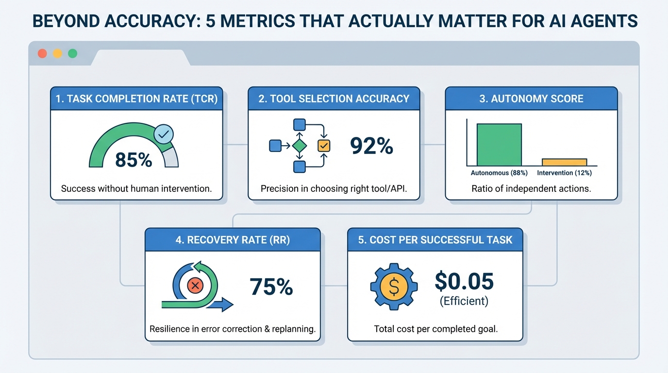
Beyond Accuracy: 5 Metrics That Actually Matter for AI AgentsImage by Editor Introduction AI agents, or autonomous systems powered by agentic AI, have reshaped the current landscape of AI systems and deployments. As these systems become more capable, we also need specialized evaluation metrics that quantify not only correctness, but also procedural reasoning, reliability, and efficiency. While accuracy is one of the most common metrics used in static large language model evaluations, agent evaluations often require additional measures focused on action quality, tool use, and trajectory efficiency — especially when building modern AI agents. This article lists five such metrics, along with further readings to dive deeper into each. 1. Task Completion Rate (TCR) Also known as Success Rate, this metric measures the percentage of assigned tasks that are successfully carried out without the need for human supervision or intervention. Think of it as a measure of the agent’s ability to connect reasoning to a correct final outcome. For example, a customer support bot resolving a refund issue on its own could count toward this metric. Be warned: using this metric as a binary measure (success vs. failure) by itself can mask borderline cases or tasks that technically succeeded but took prohibitively long to complete. Read more in this paper. 2. Tool Selection Accuracy This measures how precisely the agent selects and executes the right function, external component, or API at a given step — in other words, how consistently it makes good selection-oriented decisions instead of acting randomly. Action selection becomes especially important in high-stakes domains like finance. To use this metric properly, you typically need a “ground truth” or “gold standard” path to compare against, which can be tricky to define in some contexts. Read more in this overview. 3. Autonomy Score Also referred to as the Human Intervention Rate, this is the ratio of actions taken autonomously by the agent to those that required some form of human intervention (clarification, correction, approvals, and so on). It is strongly related to the return on investment (ROI) of using AI agents. Bear in mind, though, that in critical domains like healthcare, low autonomy is not necessarily a bad thing. In fact, pushing autonomy too high can be a sign that safety guardrails are missing, so this metric must be interpreted in the context of the application. Read more in this Anthropic research post. 4. Recovery Rate (RR) How frequently does an agent identify an error and effectively replan to fix it? That is the core idea behind recovery rate: a metric for an agent’s resilience to unexpected outcomes, especially when it frequently interacts with tools and external systems outside its direct control. It requires careful interpretation, since a very high recovery rate can sometimes reveal underlying instability if the agent is correcting itself almost all the time. Read more in this paper. 5. Cost per Successful Task This metric is also described using names like token efficiency and cost-per-goal, but in essence, it measures the total computational or economic cost invested to complete one task successfully. This is an important metric to watch when planning to scale agent-based systems to handle higher volumes of tasks without cost surprises. Read more in this guide. About Iván Palomares Carrascosa Iván Palomares Carrascosa is a leader, writer, speaker, and adviser in AI, machine learning, deep learning & LLMs. He trains and guides others in harnessing AI in the real world.
Access Denied
Access Denied You don’t have permission to access “http://zeenews.india.com/technology/whatsapp-payment-scam-how-to-stay-safe-from-fake-requests-links-and-qr-codes-3025239.html” on this server. Reference #18.85277368.1773039880.5fb3629 https://errors.edgesuite.net/18.85277368.1773039880.5fb3629
Introduction to Small Language Models: The Complete Guide for 2026
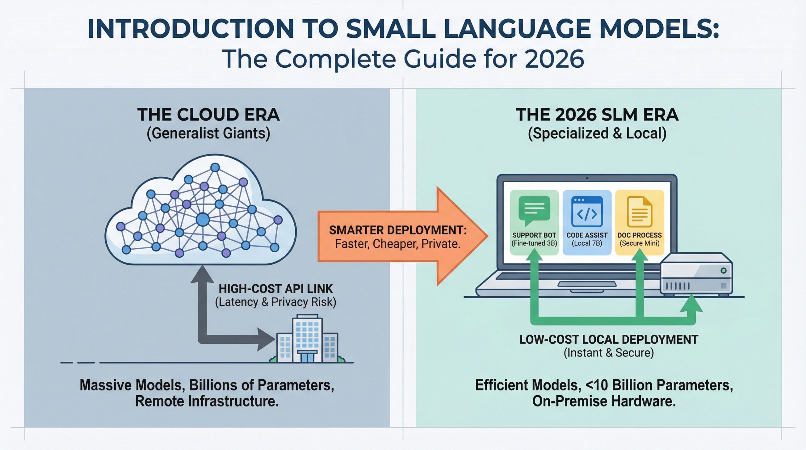
In this article, you will learn what small language models are, why they matter in 2026, and how to use them effectively in real production systems. Topics we will cover include: What defines small language models and how they differ from large language models. The cost, latency, and privacy advantages driving SLM adoption. Practical use cases and a clear path to getting started. Let’s get straight to it. Introduction to Small Language Models: The Complete Guide for 2026Image by Author Introduction AI deployment is changing. While headlines focus on ever-larger language models breaking new benchmarks, production teams are discovering that smaller models can handle most everyday tasks at a fraction of the cost. If you’ve deployed a chatbot, built a code assistant, or automated document processing, you’ve probably paid for cloud API calls to models with hundreds of billions of parameters. But most practitioners working in 2026 are finding that for 80% of production use cases, a model you can run on a laptop works just as well and costs 95% less. If you want to jump straight into hands-on options, our guide to the Top 7 Small Language Models You Can Run on a Laptop covers the best models available today and how to get them running locally. Small language models (SLMs) make this possible. This guide covers what they are, when to use them, and how they’re changing the economics of AI deployment. What Are Small Language Models? Small language models are language models with fewer than 10 billion parameters, usually ranging from 1 billion to 7 billion. Parameters are the “knobs and dials” inside a neural network. Each parameter is a numerical value the model uses to transform input text into predictions about what comes next. When you see “GPT-4 has over 1 trillion parameters,” that means the model has 1 trillion of these adjustable values working together to understand and generate language. More parameters generally mean more capacity to learn patterns, but they also mean more computational power, memory, and cost to run. The scale difference is significant. GPT-4 has over 1 trillion parameters, Claude Opus has hundreds of billions, and even Llama 3.1 70B is considered “large.” SLMs operate at a completely different scale. But “small” doesn’t mean “simple.” Modern SLMs like Phi-3 Mini (3.8B parameters), Llama 3.2 3B, and Mistral 7B deliver performance that rivals models 10× their size on many tasks. The real difference is specialization. Where large language models are trained to be generalists with broad knowledge spanning every topic imaginable, SLMs excel when fine-tuned for specific domains. A 3B model trained on customer support conversations will outperform GPT-4 on your specific support queries while running on hardware you already own. You Don’t Build Them From Scratch Adopting an SLM doesn’t mean building one from the ground up. Even “small” models are far too complex for individuals or small teams to train from scratch. Instead, you download a pre-trained model that already understands language, then teach it your specific domain through fine-tuning. It’s like hiring an employee who already speaks English and training them on your company’s procedures, rather than teaching a baby to speak from birth. The model arrives with general language understanding built in. You’re just adding specialized knowledge. You don’t need a team of PhD researchers or massive computing clusters. You need a developer with Python skills, some example data from your domain, and a few hours of GPU time. The barrier to entry is much lower than most people assume. Why SLMs Matter in 2026 Three forces are driving SLM adoption: cost, latency, and privacy. Cost: Cloud API pricing for large models runs \$0.01 to \$0.10 per 1,000 tokens. At scale, this adds up fast. A customer support system handling 100,000 queries per day can rack up $30,000+ monthly in API costs. An SLM running on a single GPU server costs the same hardware whether it processes 10,000 or 10 million queries. The economics flip entirely. Latency: When you call a cloud API, you’re waiting for network round-trips plus inference time. SLMs running locally respond in 50 to 200 milliseconds. For applications like coding assistants or interactive chatbots, users feel this difference immediately. Privacy: Regulated industries (healthcare, finance, legal) can’t send sensitive data to external APIs. SLMs let these organizations deploy AI while keeping data on-premise. No external API calls means no data leaves your infrastructure. LLMs vs SLMs: Understanding the Trade-offs The decision between an LLM and an SLM depends on matching capability to requirements. The differences come down to scale, deployment model, and the nature of the task. The comparison reveals a pattern: LLMs are designed for breadth and unpredictability, while SLMs are built for depth and repetition. If your task requires handling any question about any topic, you need an LLM’s broad knowledge. But if you’re solving the same type of problem thousands of times, an SLM fine-tuned for that specific domain will be faster, cheaper, and often more accurate. Here’s a concrete example. If you’re building a legal document analyzer, an LLM can handle any legal question from corporate law to international treaties. But if you’re only processing employment contracts, a fine-tuned 7B model will be faster, cheaper, and more accurate on that specific task. Most teams are landing on a hybrid approach: use SLMs for 80% of queries (the predictable ones), escalate to LLMs for the complex 20%. This “router” pattern combines the best of both worlds. How SLMs Achieve Their Edge SLMs aren’t just “small LLMs.” They use specific techniques to deliver high performance at low parameter counts. Knowledge Distillation trains smaller “student” models to mimic larger “teacher” models. The student learns to replicate the teacher’s outputs without needing the same massive architecture. Microsoft’s Phi-3 series was distilled from much larger models, retaining 90%+ of the capability at 5% of the size. High-Quality Training Data matters more for SLMs than sheer data quantity. While LLMs are trained on trillions of tokens from the entire internet, SLMs benefit from curated, high-quality
Access Denied
Access Denied You don’t have permission to access “http://zeenews.india.com/technology/bharatnet-connects-2-15-lakh-gram-panchayats-4-09-lakh-hotspots-expand-rural-digital-connectivity-3024933.html” on this server. Reference #18.eff43717.1773024574.5c96fb37 https://errors.edgesuite.net/18.eff43717.1773024574.5c96fb37
Build Semantic Search with LLM Embeddings
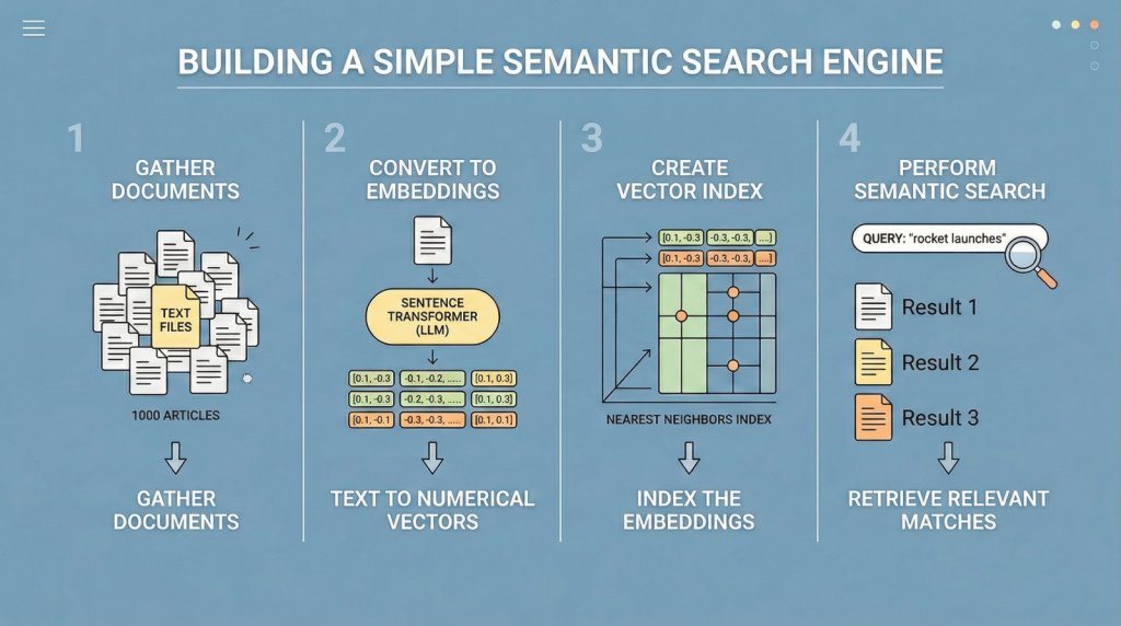
In this article, you will learn how to build a simple semantic search engine using sentence embeddings and nearest neighbors. Topics we will cover include: Understanding the limitations of keyword-based search. Generating text embeddings with a sentence transformer model. Implementing a nearest-neighbor semantic search pipeline in Python. Let’s get started. Build Semantic Search with LLM EmbeddingsImage by Editor Introduction Traditional search engines have historically relied on keyword search. In other words, given a query like “best temples and shrines to visit in Fukuoka, Japan”, results are retrieved based on keyword matching, such that text documents containing co-occurrences of words like “temple”, “shrine”, and “Fukuoka” are deemed most relevant. However, this classical approach is notoriously rigid, as it largely relies on exact word matches and misses other important semantic nuances such as synonyms or alternative phrasing — for example, “young dog” instead of “puppy”. As a result, highly relevant documents may be inadvertently omitted. Semantic search addresses this limitation by focusing on meaning rather than exact wording. Large language models (LLMs) play a key role here, as some of them are trained to translate text into numerical vector representations called embeddings, which encode the semantic information behind the text. When two texts like “small dogs are very curious by nature” and “puppies are inquisitive by nature” are converted into embedding vectors, those vectors will be highly similar due to their shared meaning. Meanwhile, the embedding vectors for “puppies are inquisitive by nature” and “Dazaifu is a signature shrine in Fukuoka” will be very different, as they represent unrelated concepts. Following this principle — which you can explore in more depth here — the remainder of this article guides you through the full process of building a compact yet efficient semantic search engine. While minimalistic, it performs effectively and serves as a starting point for understanding how modern search and retrieval systems, such as retrieval augmented generation (RAG) architectures, are built. The code explained below can be run seamlessly in a Google Colab or Jupyter Notebook instance. Step-by-Step Guide First, we make the necessary imports for this practical example: import pandas as pd import json from pydantic import BaseModel, Field from openai import OpenAI from google.colab import userdata from sklearn.ensemble import RandomForestClassifier from sklearn.model_selection import train_test_split from sklearn.metrics import classification_report from sklearn.preprocessing import StandardScaler import pandas as pd import json from pydantic import BaseModel, Field from openai import OpenAI from google.colab import userdata from sklearn.ensemble import RandomForestClassifier from sklearn.model_selection import train_test_split from sklearn.metrics import classification_report from sklearn.preprocessing import StandardScaler We will use a toy public dataset called “ag_news”, which contains texts from news articles. The following code loads the dataset and selects the first 1000 articles. from datasets import load_dataset from sentence_transformers import SentenceTransformer from sklearn.neighbors import NearestNeighbors from datasets import load_dataset from sentence_transformers import SentenceTransformer from sklearn.neighbors import NearestNeighbors We now load the dataset and extract the “text” column, which contains the article content. Afterwards, we print a short sample from the first article to inspect the data: print(“Loading dataset…”) dataset = load_dataset(“ag_news”, split=”train[:1000]”) # Extract the text column into a Python list documents = dataset[“text”] print(f”Loaded {len(documents)} documents.”) print(f”Sample: {documents[0][:100]}…”) print(“Loading dataset…”) dataset = load_dataset(“ag_news”, split=“train[:1000]”) # Extract the text column into a Python list documents = dataset[“text”] print(f“Loaded {len(documents)} documents.”) print(f“Sample: {documents[0][:100]}…”) The next step is to obtain embedding vectors (numerical representations) for our 1000 texts. As mentioned earlier, some LLMs are trained specifically to translate text into numerical vectors that capture semantic characteristics. Hugging Face sentence transformer models, such as “all-MiniLM-L6-v2″, are a common choice. The following code initializes the model and encodes the batch of text documents into embeddings. print(“Loading embedding model…”) model = SentenceTransformer(“all-MiniLM-L6-v2”) # Convert text documents into numerical vector embeddings print(“Encoding documents (this may take a few seconds)…”) document_embeddings = model.encode(documents, show_progress_bar=True) print(f”Created {document_embeddings.shape[0]} embeddings.”) print(“Loading embedding model…”) model = SentenceTransformer(“all-MiniLM-L6-v2”) # Convert text documents into numerical vector embeddings print(“Encoding documents (this may take a few seconds)…”) document_embeddings = model.encode(documents, show_progress_bar=True) print(f“Created {document_embeddings.shape[0]} embeddings.”) Next, we initialize a NearestNeighbors object, which implements a nearest-neighbor strategy to find the k most similar documents to a given query. In terms of embeddings, this means identifying the closest vectors (smallest angular distance). We use the cosine metric, where more similar vectors have smaller cosine distances (and higher cosine similarity values). search_engine = NearestNeighbors(n_neighbors=5, metric=”cosine”) search_engine.fit(document_embeddings) print(“Search engine is ready!”) search_engine = NearestNeighbors(n_neighbors=5, metric=“cosine”) search_engine.fit(document_embeddings) print(“Search engine is ready!”) The core logic of our search engine is encapsulated in the following function. It takes a plain-text query, specifies how many top results to retrieve via top_k, computes the query embedding, and retrieves the nearest neighbors from the index. The loop inside the function prints the top-k results ranked by similarity: def semantic_search(query, top_k=3): # Embed the incoming search query query_embedding = model.encode([query]) # Retrieve the closest matches distances, indices = search_engine.kneighbors(query_embedding, n_neighbors=top_k) print(f”\n🔍 Query: ‘{query}’”) print(“-” * 50) for i in range(top_k): doc_idx = indices[0][i] # Convert cosine distance to similarity (1 – distance) similarity = 1 – distances[0][i] print(f”Result {i+1} (Similarity: {similarity:.4f})”) print(f”Text: {documents[int(doc_idx)][:150]}…\n”) 1 2 3 4 5 6 7 8 9 10 11 12 13 14 15 16 17 def semantic_search(query, top_k=3): # Embed the incoming search query query_embedding = model.encode([query]) # Retrieve the closest matches distances, indices = search_engine.kneighbors(query_embedding, n_neighbors=top_k) print(f“\n🔍 Query: ‘{query}’”) print(“-“ * 50) for i in range(top_k): doc_idx = indices[0][i] # Convert cosine distance to similarity (1 – distance) similarity = 1 – distances[0][i] print(f“Result {i+1} (Similarity: {similarity:.4f})”) print(f“Text: {documents[int(doc_idx)][:150]}…\n”) And that’s it. To test the function, we can formulate a couple of example search queries: semantic_search(“Wall street and stock market trends”) semantic_search(“Space exploration and rocket launches”) semantic_search(“Wall street and stock market trends”) semantic_search(“Space exploration and rocket launches”) The results are ranked by similarity (truncated here for clarity): 🔍 Query: ‘Wall street and stock market trends’ ————————————————– Result 1 (Similarity: 0.6258) Text: Stocks Higher Despite Soaring Oil Prices NEW YORK – Wall
Access Denied
Access Denied You don’t have permission to access “http://zeenews.india.com/technology/watching-ind-vs-nz-t20-world-cup-2026-final-online-5-tips-for-faster-internet-speed-and-buffer-free-match-streaming-3024914.html” on this server. Reference #18.f42ddf17.1772963264.1dd65afc https://errors.edgesuite.net/18.f42ddf17.1772963264.1dd65afc
Deploying AI Agents to Production: Architecture, Infrastructure, and Implementation Roadmap
Deploying AI Agents to Production: Architecture, Infrastructure, and Implementation Roadmap – MachineLearningMastery.com Deploying AI Agents to Production: Architecture, Infrastructure, and Implementation Roadmap – MachineLearningMastery.com