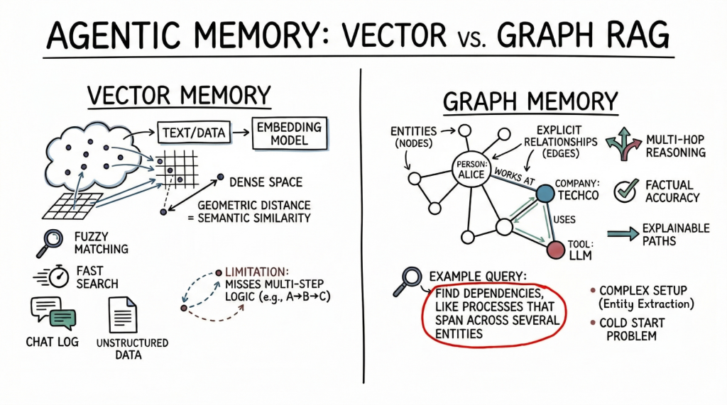
In this article, you will learn how vector databases and graph RAG differ as memory architectures for AI agents, and when each approach is the better fit. Topics we will cover include: How vector databases store and retrieve semantically similar unstructured information. How graph RAG represents entities and relationships for precise, multi-hop retrieval. How to choose between these approaches, or combine them in a hybrid agent-memory architecture. With that in mind, let’s get straight to it. Vector Databases vs. Graph RAG for Agent Memory: When to Use WhichImage by Author Introduction AI agents need long-term memory to be genuinely useful in complex, multi-step workflows. An agent without memory is essentially a stateless function that resets its context with every interaction. As we move toward autonomous systems that manage persistent tasks (such as like coding assistants that track project architecture or research agents that compile ongoing literature reviews) the question of how to store, retrieve, and update context becomes critical. Currently, the industry standard for this task is the vector database, which uses dense embeddings for semantic search. Yet, as the need for more complex reasoning grows, graph RAG, an architecture that combines knowledge graphs with large language models (LLMs), is gaining traction as a structured memory architecture. At a glance, vector databases are ideal for broad similarity matching and unstructured data retrieval, while graph RAG excels when context windows are limited and when multi-hop relationships, factual accuracy, and complex hierarchical structures are required. This distinction highlights vector databases’ focus on flexible matching, compared with graph RAG’s ability to reason through explicit relationships and preserve accuracy under tighter constraints. To clarify their respective roles, this article explores the underlying theory, practical strengths, and limitations of both approaches for agent memory. In doing so, it provides a practical framework to guide the choice of system, or combination of systems, to deploy. Vector Databases: The Foundation of Semantic Agent Memory Vector databases represent memory as dense mathematical vectors, or embeddings, situated in high-dimensional space. An embedding model maps text, images, or other data to arrays of floats, where the geometric distance between two vectors corresponds to their semantic similarity. AI agents primarily use this approach to store unstructured text. A common use case is storing conversational history, allowing the agent to recall what a user previously asked by searching its memory bank for semantically related past interactions. Agents also leverage vector stores to retrieve relevant documents, API documentation, or code snippets based on the implicit meaning of a user’s prompt, which is a far more robust approach than relying on exact keyword matches. Vector databases are strong choices for agent memory. They offer fast search, even across billions of vectors. Developers also find them easier to set up than structured databases. To integrate a vector store, you split the text, generate embeddings, and index the results. These databases also handle fuzzy matching well, accommodating typos and paraphrasing without requiring strict queries. But semantic search has limits for advanced agent memory. Vector databases often cannot follow multi-step logic. For instance, if an agent needs to find the link between entity A and entity C but only has data showing that A connects to B and B connects to C, a simple similarity search may miss important information. These databases also struggle when retrieving large amounts of text or dealing with noisy results. With dense, interconnected facts (from software dependencies to company organizational charts) they can return related but irrelevant information. This can crowd the agent’s context window with less useful data. Graph RAG: Structured Context and Relational Memory Graph RAG addresses the limitations of semantic search by combining knowledge graphs with LLMs. In this paradigm, memory is structured as discrete entities represented as nodes (for example, a person, a company, or a technology), and the explicit relationships between them are represented as edges (for example, “works at” or “uses”). Agents using graph RAG create and update a structured world model. As they gather new information, they extract entities and relationships and add them to the graph. When searching memory, they follow explicit paths to retrieve the exact context. The main strength of graph RAG is its precision. Because retrieval follows explicit relationships rather than semantic closeness alone, the risk of error is lower. If a relationship does not exist in the graph, the agent cannot infer it from the graph alone. Graph RAG excels at complex reasoning and is ideal for answering structured questions. To find the direct reports of a manager who approved a budget, you trace a path through the organization and approval chain — a simple graph traversal, but a difficult task for vector search. Explainability is another major advantage. The retrieval path is a clear, auditable sequence of nodes and edges, not an opaque similarity score. This matters for enterprise applications that require compliance and transparency. On the downside, graph RAG introduces significant implementation complexity. It demands robust entity-extraction pipelines to parse raw text into nodes and edges, which often requires carefully tuned prompts, rules, or specialized models. Developers must also design and maintain an ontology or schema, which can be rigid and difficult to evolve as new domains are encountered. The cold-start problem is also prominent: unlike a vector database, which is useful the moment you embed text, a knowledge graph requires substantial upfront effort to populate before it can answer complex queries. The Comparison Framework: When to Use Which When architecting memory for an AI agent, keep in mind that vector databases excel at handling unstructured, high-dimensional data and are well suited to similarity search, whereas graph RAG is advantageous for representing entities and explicit relationships when those relationships are crucial. The choice should be driven by the data’s inherent structure and the expected query patterns. Vector databases are ideally suited to purely unstructured data — chat logs, general documentation, or sprawling knowledge bases built from raw text. They excel when the query intent is to explore broad themes, such as “Find me concepts similar to X”

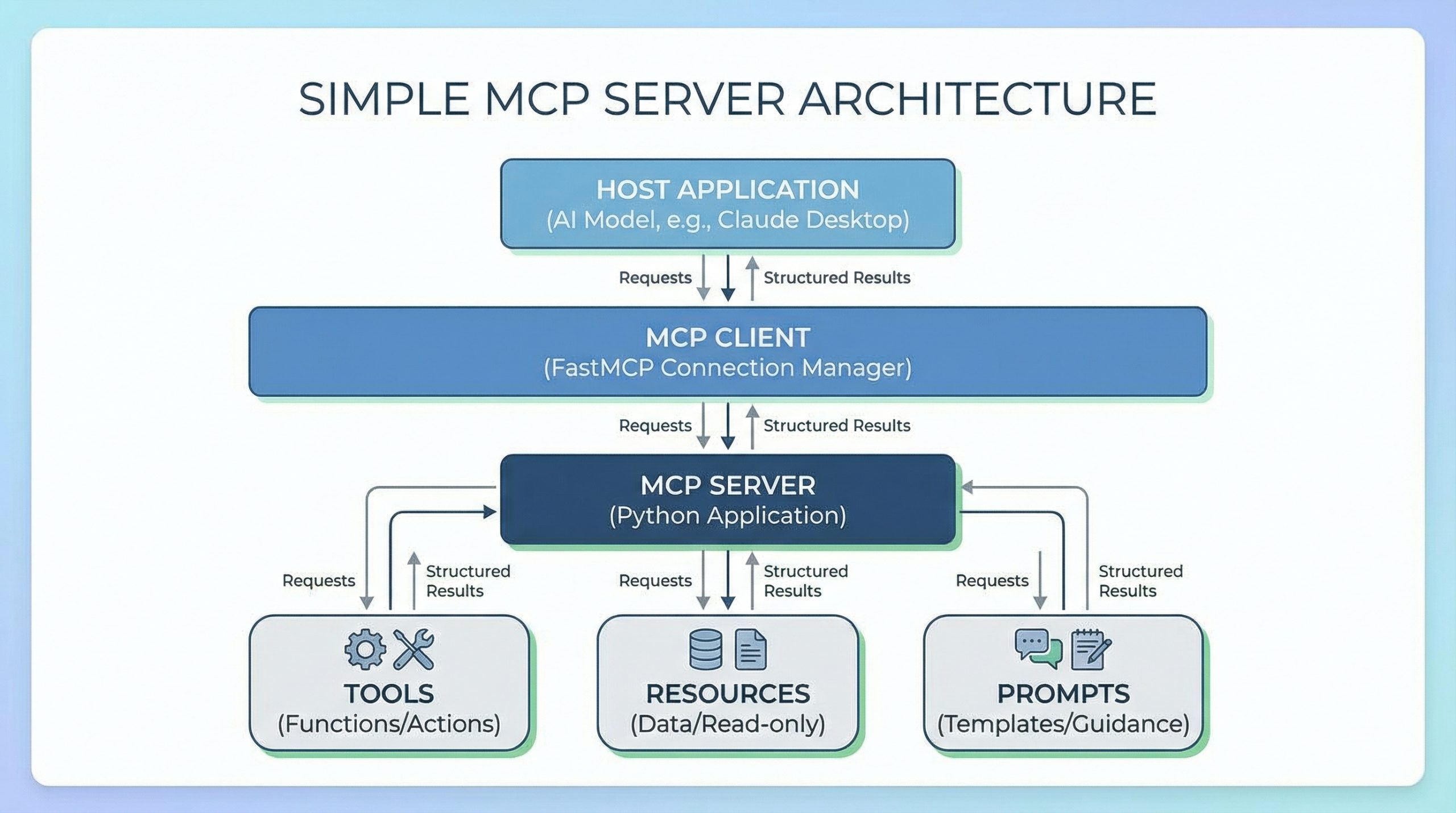
In this article, you will learn what Model Context Protocol (MCP) is and how to build a simple, practical task-tracker MCP server in Python using FastMCP. Topics we will cover include: How MCP works, including hosts, clients, servers, and the three core primitives. How to implement MCP tools, resources, and prompts with FastMCP. How to run and test your MCP server using the FastMCP client. Let’s not waste any more time. Building a Simple MCP Server in PythonImage by Editor Introduction Have you ever tried connecting a language model to your own data or tools? If so, you know it often means writing custom integrations, managing API schemas, and wrestling with authentication. And every new AI application can feel like rebuilding the same connection logic from scratch. Model Context Protocol (MCP) solves this by standardizing how large language models (LLMs) and other AI models interact with external systems. FastMCP is a framework that makes building MCP servers simple. In this article, you’ll learn what MCP is, how it works, and how to build a practical task tracker server using FastMCP. You’ll create tools to manage tasks, resources to view task lists, and prompts to guide AI interactions. You can get the code on GitHub. Understanding the Model Context Protocol As mentioned, Model Context Protocol (MCP) is an open protocol that defines how AI applications communicate with external systems. How MCP Works MCP has three components: Hosts are the AI-powered applications users actually interact with. The host can be Claude Desktop, an IDE with AI features, or a custom app you’ve built. The host contains (or interfaces with) the language model and initiates connections to MCP servers. Clients connect to servers. When a host needs to talk to an MCP server, it creates a client instance to manage that specific connection. One host can run multiple clients simultaneously, each connected to a different server. The client handles all protocol-level communication. Servers are what you build. They expose specific capabilities — database access, file operations, API integrations — and respond to client requests by providing tools, resources, and prompts. So the user interacts with the host, the host uses a client to talk to your server, and the server returns structured results back up the chain. To learn more about MCP, read The Complete Guide to Model Context Protocol. The Three Core Primitives MCP servers expose three types of functionality: Tools are functions that perform actions. They’re like executable commands the LLM can invoke. add_task, send_an_email, and query_a_database are some examples of tools. Resources provide read-only access to data. They allow viewing information without changing it. Examples include lists of tasks, configuration files, and user profiles. Prompts are templates that guide AI interactions. They structure how the model approaches specific tasks. Examples include “Analyze these tasks and suggest priorities” and “Review this code for security issues.” In practice, you’ll combine these primitives. An AI model might use a resource to view tasks, then a tool to update one, guided by a prompt that defines the workflow. Setting Up Your Environment You’ll need Python 3.10 or later. Install FastMCP using pip (or uv if you prefer): Let’s get started! Building a Task Tracker Server We’ll build a server that manages a simple task list. Create a file called task_server.py and add the imports: from fastmcp import FastMCP from datetime import datetime from fastmcp import FastMCP from datetime import datetime These give us the FastMCP framework and datetime handling for tracking when tasks were created. Initializing the Server Now set up the server and a simple in-memory storage: mcp = FastMCP(“TaskTracker”) # Simple in-memory task storage tasks = [] task_id_counter = 1 mcp = FastMCP(“TaskTracker”)   # Simple in-memory task storage tasks = [] task_id_counter = 1 Here’s what this does: FastMCP(“TaskTracker”) creates your MCP server with a descriptive name. tasks is a list that stores all tasks. task_id_counter generates unique IDs for each task. In a real application, you’d use a database. For this tutorial, we’ll keep it simple. Creating Tools Tools are functions decorated with @mcp.tool(). Let’s create three useful tools. Tool 1: Adding a New Task First, let’s create a tool that adds tasks to our list: @mcp.tool() def add_task(title: str, description: str = “”) -> dict: “””Add a new task to the task list.””” global task_id_counter task = { “id”: task_id_counter, “title”: title, “description”: description, “status”: “pending”, “created_at”: datetime.now().isoformat() } tasks.append(task) task_id_counter += 1 return task 1 2 3 4 5 6 7 8 9 10 11 12 13 14 15 16 17 @mcp.tool() def add_task(title: str, description: str = “”) -> dict:     “”“Add a new task to the task list.”“”     global task_id_counter          task = {         “id”: task_id_counter,         “title”: title,         “description”: description,         “status”: “pending”,         “created_at”: datetime.now().isoformat()     }          tasks.append(task)     task_id_counter += 1          return task This tool does the following: Takes a task title (required) and an optional description. Creates a task dictionary with a unique ID, status, and timestamp. Adds it to our tasks list. Returns the created task. The model can now call add_task(“Write documentation”, “Update API docs”) and get a structured task object back. Tool 2: Completing a Task Next, let’s add a tool to mark tasks as complete: @mcp.tool() def complete_task(task_id: int) -> dict: “””Mark a task as completed.””” for task in tasks: if task[“id”] == task_id: task[“status”] = “completed” task[“completed_at”] = datetime.now().isoformat() return task return {“error”: f”Task {task_id} not found”} @mcp.tool() def complete_task(task_id: int) -> dict:     “”“Mark a task as completed.”“”     for task in tasks:         if task[“id”] == task_id:             task[“status”] = “completed”             task[“completed_at”] = datetime.now().isoformat()             return task          return {“error”: f“Task {task_id} not found”} The tool searches the task list for a matching ID, updates its status to “completed”, and stamps it with a completion timestamp. It then returns the updated task or an error message if no match is found. Tool 3: Deleting a Task Finally, add a tool to remove tasks: @mcp.tool() def delete_task(task_id: int) -> dict: “””Delete a task from the list.””” for i, task

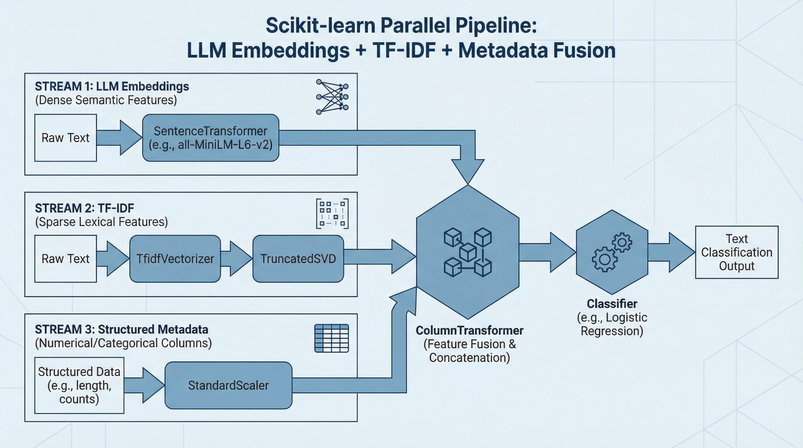
In this article, you will learn how to fuse dense LLM sentence embeddings, sparse TF-IDF features, and structured metadata into a single scikit-learn pipeline for text classification. Topics we will cover include: Loading and preparing a text dataset alongside synthetic metadata features. Building parallel feature pipelines for TF-IDF, LLM embeddings, and numeric metadata. Fusing all feature branches with ColumnTransformer and training an end-to-end classifier. Let’s break it down. How to Combine LLM Embeddings + TF-IDF + Metadata in One Scikit-learn Pipeline (click to enlarge)Image by Editor Introduction Data fusion, or combining diverse pieces of data into a single pipeline, sounds ambitious enough. If we talk not just about two, but about three complementary feature sources, then the challenge — and the potential payoff — goes to the next level. The most exciting part is that scikit-learn allows us to unify all of them cleanly within a single, end-to-end workflow. Do you want to see how? This article walks you step by step through building a complete fusion pipeline from scratch for a downstream text classification task, combining dense semantic information from LLM-generated embeddings, sparse lexical features from TF-IDF, and structured metadata signals. Interested? Keep reading. Step-by-Step Pipeline Building Process First, we will make all the necessary imports for the pipeline-building process. If you are working in a local environment, you might need to pip install some of them first: import numpy as np import pandas as pd from sklearn.datasets import fetch_20newsgroups from sklearn.model_selection import train_test_split from sklearn.pipeline import Pipeline from sklearn.compose import ColumnTransformer from sklearn.feature_extraction.text import TfidfVectorizer from sklearn.preprocessing import StandardScaler from sklearn.linear_model import LogisticRegression from sklearn.metrics import classification_report from sklearn.base import BaseEstimator, TransformerMixin from sklearn.decomposition import TruncatedSVD from sentence_transformers import SentenceTransformer import numpy as np import pandas as pd   from sklearn.datasets import fetch_20newsgroups from sklearn.model_selection import train_test_split from sklearn.pipeline import Pipeline from sklearn.compose import ColumnTransformer from sklearn.feature_extraction.text import TfidfVectorizer from sklearn.preprocessing import StandardScaler from sklearn.linear_model import LogisticRegression from sklearn.metrics import classification_report from sklearn.base import BaseEstimator, TransformerMixin from sklearn.decomposition import TruncatedSVD   from sentence_transformers import SentenceTransformer Let’s look closely at this — almost endless! — list of imports. I bet one element has caught your attention: fetch_20newsgroups. This is a freely available text dataset in scikit-learn that we will use throughout this article: it contains text extracted from news articles belonging to a wide variety of categories. To keep our dataset manageable in practice, we will pick the news articles belonging to a subset of categories specified by us. The following code does the trick: categories = [ “rec.sport.baseball”, “sci.space”, “comp.graphics”, “talk.politics.misc” ] dataset = fetch_20newsgroups( subset=”all”, categories=categories, remove=(“headers”, “footers”, “quotes”) ) X_raw = dataset.data y = dataset.target print(f”Number of samples: {len(X_raw)}”) 1 2 3 4 5 6 7 8 9 10 11 12 13 14 15 16 17 categories = [     “rec.sport.baseball”,     “sci.space”,     “comp.graphics”,     “talk.politics.misc” ]   dataset = fetch_20newsgroups(     subset=“all”,     categories=categories,     remove=(“headers”, “footers”, “quotes”) )   X_raw = dataset.data y = dataset.target   print(f“Number of samples: {len(X_raw)}”) We called this freshly created dataset X_raw to emphasize that this is a raw, far-from-final version of the dataset we will gradually construct for downstream tasks like using machine learning models for predictive purposes. It is fair to say that the “raw” suffix is also used because here we have the raw text, from which three different data components (or streams) will be generated and later merged. For the structured metadata associated with the news articles obtained, in real-world contexts, this metadata might already be available or provided by the dataset owner. That’s not the case with this publicly available dataset, so we will synthetically create some simple metadata features based on the text, including features describing character length, word count, average word length, uppercase ratio, and digit ratio. def generate_metadata(texts): lengths = [len(t) for t in texts] word_counts = [len(t.split()) for t in texts] avg_word_lengths = [] uppercase_ratios = [] digit_ratios = [] for t in texts: words = t.split() if words: avg_word_lengths.append(np.mean([len(w) for w in words])) else: avg_word_lengths.append(0) denom = max(len(t), 1) uppercase_ratios.append( sum(1 for c in t if c.isupper()) / denom ) digit_ratios.append( sum(1 for c in t if c.isdigit()) / denom ) return pd.DataFrame({ “text”: texts, “char_length”: lengths, “word_count”: word_counts, “avg_word_length”: avg_word_lengths, “uppercase_ratio”: uppercase_ratios, “digit_ratio”: digit_ratios }) # Calling the function to generate a structured dataset that contains: raw text + metadata df = generate_metadata(X_raw) df[“target”] = y df.head() 1 2 3 4 5 6 7 8 9 10 11 12 13 14 15 16 17 18 19 20 21 22 23 24 25 26 27 28 29 30 31 32 33 34 35 36 37 38 39 def generate_metadata(texts):     lengths = [len(t) for t in texts]     word_counts = [len(t.split()) for t in texts]          avg_word_lengths = []     uppercase_ratios = []     digit_ratios = []       for t in texts:         words = t.split()         if words:             avg_word_lengths.append(np.mean([len(w) for w in words]))         else:             avg_word_lengths.append(0)           denom = max(len(t), 1)           uppercase_ratios.append(             sum(1 for c in t if c.isupper()) / denom         )           digit_ratios.append(             sum(1 for c in t if c.isdigit()) / denom         )       return pd.DataFrame({         “text”: texts,         “char_length”: lengths,         “word_count”: word_counts,         “avg_word_length”: avg_word_lengths,         “uppercase_ratio”: uppercase_ratios,         “digit_ratio”: digit_ratios     })   # Calling the function to generate a structured dataset that contains: raw text + metadata df = generate_metadata(X_raw) df[“target”] = y   df.head() Before getting fully into the pipeline-building process, we will split the data into train and test subsets: X = df.drop(columns=[“target”]) y = df[“target”] X_train, X_test, y_train, y_test = train_test_split( X, y, test_size=0.2, random_state=42, stratify=y ) X = df.drop(columns=[“target”]) y = df[“target”]   X_train, X_test, y_train, y_test = train_test_split(     X, y, test_size=0.2, random_state=42, stratify=y ) Very important: splitting the data into training and test sets must be done before extracting the LLM embeddings and TF-IDF features. Why? Because these two extraction processes become part of the pipeline, and they involve fitting transformations with scikit-learn, which are learning processes — for example, learning the TF-IDF vocabulary and inverse document frequency (IDF) statistics. The