Access Denied You don’t have permission to access “http://zeenews.india.com/technology/what-is-anthropic-ai-how-it-helped-u-s-israel-to-kill-iran-s-supreme-leader-ali-khamenei-3023900.html” on this server. Reference #18.eff43717.1772720769.3c503192 https://errors.edgesuite.net/18.eff43717.1772720769.3c503192
Access Denied
Access Denied You don’t have permission to access “http://zeenews.india.com/technology/ai-6g-quantum-computing-to-drive-india-finland-strategic-partnership-pm-modi-3024037.html” on this server. Reference #18.f42ddf17.1772712327.1403c7b9 https://errors.edgesuite.net/18.f42ddf17.1772712327.1403c7b9
Access Denied
Access Denied You don’t have permission to access “http://zeenews.india.com/technology/apple-m5-pro-vs-m5-max-both-chips-may-look-similar-but-they-arent-key-differences-explained-3023878.html” on this server. Reference #18.d42fdf17.1772691321.24a2445 https://errors.edgesuite.net/18.d42fdf17.1772691321.24a2445
Access Denied
Access Denied You don’t have permission to access “http://zeenews.india.com/technology/x-to-suspend-revenue-sharing-for-users-posting-undisclosed-ai-war-videos-3023577.html” on this server. Reference #18.c4f43717.1772618290.35c3bd7b https://errors.edgesuite.net/18.c4f43717.1772618290.35c3bd7b
Access Denied
Access Denied You don’t have permission to access “http://zeenews.india.com/technology/claude-down-anthropics-ai-tool-faces-second-outage-in-24-hours-chatgpt-uninstalls-surge-295-in-us-how-to-extract-data-from-openais-chatbot-3023266.html” on this server. Reference #18.c4f43717.1772535039.2df345f7 https://errors.edgesuite.net/18.c4f43717.1772535039.2df345f7
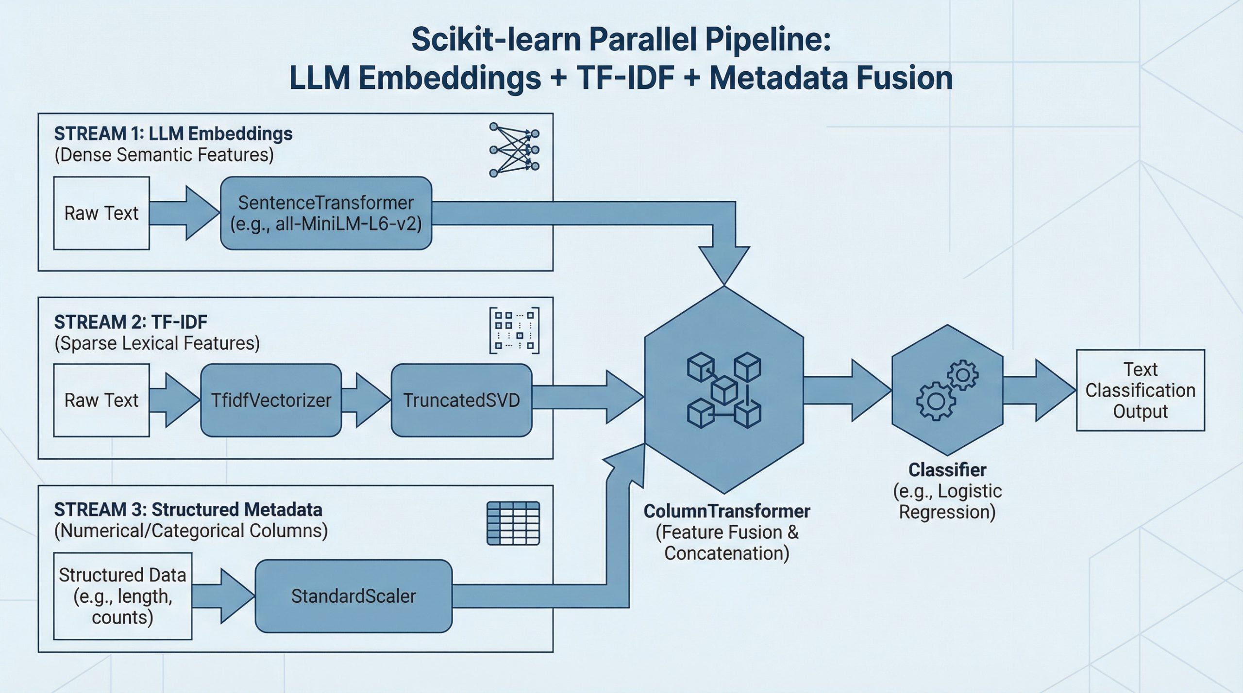
How to Combine LLM Embeddings + TF-IDF + Metadata in One Scikit-learn Pipeline
In this article, you will learn how to fuse dense LLM sentence embeddings, sparse TF-IDF features, and structured metadata into a single scikit-learn pipeline for text classification. Topics we will cover include: Loading and preparing a text dataset alongside synthetic metadata features. Building parallel feature pipelines for TF-IDF, LLM embeddings, and numeric metadata. Fusing all feature branches with ColumnTransformer and training an end-to-end classifier. Let’s break it down. How to Combine LLM Embeddings + TF-IDF + Metadata in One Scikit-learn Pipeline (click to enlarge)Image by Editor Introduction Data fusion, or combining diverse pieces of data into a single pipeline, sounds ambitious enough. If we talk not just about two, but about three complementary feature sources, then the challenge — and the potential payoff — goes to the next level. The most exciting part is that scikit-learn allows us to unify all of them cleanly within a single, end-to-end workflow. Do you want to see how? This article walks you step by step through building a complete fusion pipeline from scratch for a downstream text classification task, combining dense semantic information from LLM-generated embeddings, sparse lexical features from TF-IDF, and structured metadata signals. Interested? Keep reading. Step-by-Step Pipeline Building Process First, we will make all the necessary imports for the pipeline-building process. If you are working in a local environment, you might need to pip install some of them first: import numpy as np import pandas as pd from sklearn.datasets import fetch_20newsgroups from sklearn.model_selection import train_test_split from sklearn.pipeline import Pipeline from sklearn.compose import ColumnTransformer from sklearn.feature_extraction.text import TfidfVectorizer from sklearn.preprocessing import StandardScaler from sklearn.linear_model import LogisticRegression from sklearn.metrics import classification_report from sklearn.base import BaseEstimator, TransformerMixin from sklearn.decomposition import TruncatedSVD from sentence_transformers import SentenceTransformer import numpy as np import pandas as pd from sklearn.datasets import fetch_20newsgroups from sklearn.model_selection import train_test_split from sklearn.pipeline import Pipeline from sklearn.compose import ColumnTransformer from sklearn.feature_extraction.text import TfidfVectorizer from sklearn.preprocessing import StandardScaler from sklearn.linear_model import LogisticRegression from sklearn.metrics import classification_report from sklearn.base import BaseEstimator, TransformerMixin from sklearn.decomposition import TruncatedSVD from sentence_transformers import SentenceTransformer Let’s look closely at this — almost endless! — list of imports. I bet one element has caught your attention: fetch_20newsgroups. This is a freely available text dataset in scikit-learn that we will use throughout this article: it contains text extracted from news articles belonging to a wide variety of categories. To keep our dataset manageable in practice, we will pick the news articles belonging to a subset of categories specified by us. The following code does the trick: categories = [ “rec.sport.baseball”, “sci.space”, “comp.graphics”, “talk.politics.misc” ] dataset = fetch_20newsgroups( subset=”all”, categories=categories, remove=(“headers”, “footers”, “quotes”) ) X_raw = dataset.data y = dataset.target print(f”Number of samples: {len(X_raw)}”) 1 2 3 4 5 6 7 8 9 10 11 12 13 14 15 16 17 categories = [ “rec.sport.baseball”, “sci.space”, “comp.graphics”, “talk.politics.misc” ] dataset = fetch_20newsgroups( subset=“all”, categories=categories, remove=(“headers”, “footers”, “quotes”) ) X_raw = dataset.data y = dataset.target print(f“Number of samples: {len(X_raw)}”) We called this freshly created dataset X_raw to emphasize that this is a raw, far-from-final version of the dataset we will gradually construct for downstream tasks like using machine learning models for predictive purposes. It is fair to say that the “raw” suffix is also used because here we have the raw text, from which three different data components (or streams) will be generated and later merged. For the structured metadata associated with the news articles obtained, in real-world contexts, this metadata might already be available or provided by the dataset owner. That’s not the case with this publicly available dataset, so we will synthetically create some simple metadata features based on the text, including features describing character length, word count, average word length, uppercase ratio, and digit ratio. def generate_metadata(texts): lengths = [len(t) for t in texts] word_counts = [len(t.split()) for t in texts] avg_word_lengths = [] uppercase_ratios = [] digit_ratios = [] for t in texts: words = t.split() if words: avg_word_lengths.append(np.mean([len(w) for w in words])) else: avg_word_lengths.append(0) denom = max(len(t), 1) uppercase_ratios.append( sum(1 for c in t if c.isupper()) / denom ) digit_ratios.append( sum(1 for c in t if c.isdigit()) / denom ) return pd.DataFrame({ “text”: texts, “char_length”: lengths, “word_count”: word_counts, “avg_word_length”: avg_word_lengths, “uppercase_ratio”: uppercase_ratios, “digit_ratio”: digit_ratios }) # Calling the function to generate a structured dataset that contains: raw text + metadata df = generate_metadata(X_raw) df[“target”] = y df.head() 1 2 3 4 5 6 7 8 9 10 11 12 13 14 15 16 17 18 19 20 21 22 23 24 25 26 27 28 29 30 31 32 33 34 35 36 37 38 39 def generate_metadata(texts): lengths = [len(t) for t in texts] word_counts = [len(t.split()) for t in texts] avg_word_lengths = [] uppercase_ratios = [] digit_ratios = [] for t in texts: words = t.split() if words: avg_word_lengths.append(np.mean([len(w) for w in words])) else: avg_word_lengths.append(0) denom = max(len(t), 1) uppercase_ratios.append( sum(1 for c in t if c.isupper()) / denom ) digit_ratios.append( sum(1 for c in t if c.isdigit()) / denom ) return pd.DataFrame({ “text”: texts, “char_length”: lengths, “word_count”: word_counts, “avg_word_length”: avg_word_lengths, “uppercase_ratio”: uppercase_ratios, “digit_ratio”: digit_ratios }) # Calling the function to generate a structured dataset that contains: raw text + metadata df = generate_metadata(X_raw) df[“target”] = y df.head() Before getting fully into the pipeline-building process, we will split the data into train and test subsets: X = df.drop(columns=[“target”]) y = df[“target”] X_train, X_test, y_train, y_test = train_test_split( X, y, test_size=0.2, random_state=42, stratify=y ) X = df.drop(columns=[“target”]) y = df[“target”] X_train, X_test, y_train, y_test = train_test_split( X, y, test_size=0.2, random_state=42, stratify=y ) Very important: splitting the data into training and test sets must be done before extracting the LLM embeddings and TF-IDF features. Why? Because these two extraction processes become part of the pipeline, and they involve fitting transformations with scikit-learn, which are learning processes — for example, learning the TF-IDF vocabulary and inverse document frequency (IDF) statistics. The
Access Denied
Access Denied You don’t have permission to access “http://zeenews.india.com/technology/aws-outage-in-uae-amazon-data-centre-hit-by-objects-fire-disrupts-ec2-and-rds-services-as-dubai-abu-dhabi-see-iran-strikes-3022873.html” on this server. Reference #18.eff43717.1772443212.245886df https://errors.edgesuite.net/18.eff43717.1772443212.245886df
KV Caching in LLMs: A Guide for Developers
In this article, you will learn how key-value (KV) caching eliminates redundant computation in autoregressive transformer inference to dramatically improve generation speed. Topics we will cover include: Why autoregressive generation has quadratic computational complexity How the attention mechanism produces query, key, and value representations How KV caching works in practice, including pseudocode and memory trade-offs Let’s get started. KV Caching in LLMs: A Guide for DevelopersImage by Editor Introduction Language models generate text one token at a time, reprocessing the entire sequence at each step. To generate token n, the model recomputes attention over all (n-1) previous tokens. This creates \( O(n^2) \) complexity, where computation grows quadratically with sequence length, which becomes a major bottleneck for inference speed. Key-value (KV) caching eliminates this redundancy by leveraging the fact that the key and value projections in attention do not change once computed for a token. Instead of recomputing them at each step, we cache and reuse them. In practice, this can reduce redundant computation and provide 3–5× faster inference, depending on model size and hardware. Prerequisites This article assumes you are familiar with the following concepts: Neural networks and backpropagation The transformer architecture The self-attention mechanism in transformers Matrix multiplication concepts such as dot products, transposes, and basic linear algebra If any of these feel unfamiliar, the resources below are good starting points before reading on. The Illustrated Transformer by Jay Alammar is one of the clearest visual introductions to transformers and attention available. Andrej Karpathy’s Let’s Build GPT walks through building a transformer from scratch in code. Both will give you a solid foundation to get the most out of this article. That said, this article is written to be as self-contained as possible, and many concepts will become clearer in context as you go. The Computational Problem in Autoregressive Generation Large language models use autoregressive generation — producing one token at a time — where each token depends on all previous tokens. Let’s use a simple example. Start with the input word: “Python”. Suppose the model generates: Input: “Python” Step 1: “is” Step 2: “a” Step 3: “programming” Step 4: “language” Step 5: “used” Step 6: “for” … Input: “Python” Step 1: “is” Step 2: “a” Step 3: “programming” Step 4: “language” Step 5: “used” Step 6: “for” … Here is the computational problem: to generate “programming” (token 3), the model processes “Python is a”. To generate “language” (token 4), it processes “Python is a programming”. Every new token requires reprocessing all previous tokens. Here is a breakdown of tokens that get reprocessed repeatedly: “Python” gets processed 6 times (once for each subsequent token) “is” gets processed 5 times “a” gets processed 4 times “programming” gets processed 3 times The token “Python” never changes, yet we recompute its internal representations over and over. In general, the process looks like this: Generate token 1: Process 1 position Generate token 2: Process 2 positions Generate token 3: Process 3 positions … Generate token n: Process n positions Generate token 1: Process 1 position Generate token 2: Process 2 positions Generate token 3: Process 3 positions … Generate token n: Process n positions This gives us the following complexity for generating n tokens:\[\text{Cost} = 1 + 2 + 3 + \cdots + n = \frac{n(n+1)}{2} \approx O(n^2)\] Understanding the Attention Mechanism and KV Caching Think of attention as the model deciding which words to focus on. The self-attention mechanism at the core of transformers computes: \[\text{Attention}(Q, K, V) = \text{softmax}\left(\frac{QK^T}{\sqrt{d_k}}\right)V\] The mechanism creates three representations for each token: Query (Q): Each token uses its query to search the sequence for relevant context needed to be interpreted correctly. Key (K): Each token broadcasts its key so other queries can decide how relevant it is to what they are looking for. Value (V): Once a query matches a key, the value is what actually gets retrieved and used in the output. Each token enters the attention layer as a \( d_{\text{model}} \)-dimensional vector. The projection matrices \( W_Q \), \( W_K \), and \( W_V \) — learned during training through backpropagation — map it to \( d_k \) per head, where \( d_k = d_{\text{model}} / \text{num\_heads} \). During training, the full sequence is processed at once, so Q, K, and V all have shape [seq_len, d_k], and \( QK^T \) produces a full [seq_len, seq_len] matrix with every token attending to every other token simultaneously. At inference, something more interesting happens. When generating token \( t \), only Q changes. The K and V for all previous tokens \( 1 \ldots t-1 \) are identical to what they were in the previous step. Therefore, it is possible to cache these key (K) and value (V) matrices and reuse them in subsequent steps. Hence the name KV caching. Q has shape [1, d_k] since only the current token is passed in, while K and V have shape [seq_len, d_k] and [seq_len, d_v], respectively, growing by one row each step as the new token’s K and V are appended. With these shapes in mind, here is what the formula computes: \( QK^T \) computes a dot product between the current token’s query and every cached key, producing a [1, seq_len] similarity score across the full history. \( 1/\sqrt{d_k} \) scales scores down to prevent dot products from growing too large and saturating the softmax. \( \text{softmax}(\cdot) \) converts the scaled scores into a probability distribution that sums to 1. Multiplying by V weights the value vectors by those probabilities to produce the final output. Comparing Token Generation With and Without KV Caching Let’s trace through our example with concrete numbers. We will use \( d_{\text{model}} = 4 \). Real models, however, typically use 768–4096 dimensions. Input: “Python” (1 token). Suppose the language model generates: “is a programming language”. Without KV Caching At each step, K and V are recomputed for every token in the sequence, and the cost grows as each token is added. Step Sequence K & V Computed 0 Python
Access Denied
Access Denied You don’t have permission to access “http://zeenews.india.com/technology/4g-vs-5g-vs-lte-which-network-mode-is-best-for-faster-internet-and-better-battery-life-3022562.html” on this server. Reference #18.eff43717.1772369043.1687ffd4 https://errors.edgesuite.net/18.eff43717.1772369043.1687ffd4
Access Denied
Access Denied You don’t have permission to access “http://zeenews.india.com/technology/us-israel-strike-on-iran-hits-flights-is-flightradar24-down-here-s-how-to-track-real-time-flight-status-on-live-global-map-3022212.html” on this server. Reference #18.c4f43717.1772293925.b179fe5 https://errors.edgesuite.net/18.c4f43717.1772293925.b179fe5