

New Delhi: India’s electronics exports has exceeded $47 billion, or more than Rs 4.15 lakh crore, for the first time in 2025, according to official data. As per official data, the electronics exports marked a 37 per cent rise — from $34.93 billion in the prior 12‑month period in 2024. Nearly two‑thirds of the total exports, at roughly $30 billion, came from smartphone shipments supported by the government’s production‑linked incentive (PLI) scheme, which also hit an all‑time high in 2025. Electronics exports reached $4.17 billion in December 2025, up 16.8 per cent from $3.58 billion in December 2024. Electronics exports exceeded the $4 billion mark in seven of the 12 months of 2025, underscoring sustained global demand for Indian‑made devices. The export figure of smartphones in 2025 represents about 38 per cent of the country’s smartphone exports over the past five years, according to a recent report. Add Zee News as a Preferred Source The data showed that India’s smartphone shipments abroad totalled nearly $79.03 billion from 2021 to 2025, with CY25 delivering the highest 12‑month export tally on record. Apple’s iPhone consignments accounted for roughly 75 per cent of the total during this period, valued at over $22 billion. India’s electronics exports are expected to expand further due to the semiconductor manufacturing push, Union Minister Ashwini Vaishnaw recently said. “Momentum will continue in 2026 as four semiconductor plants come into commercial production,” he said in a social media post earlier this week. Official estimates showed that electronic production reached around Rs 11.3 crore in 2024–25 period. For the first time since domestic production began in 2021, US tech giant Apple Inc’s iPhone exports from India crossed Rs 2 lakh crore in 2025, and surged nearly 85 per cent over 2024 exports, as per industry data. India became the world’s second-largest mobile phone producer, with over 99 per cent of phones sold domestically now Made in India moves up the manufacturing value chain. The smartphone PLI scheme is scheduled to conclude in March 2026, though the government is reportedly exploring ways to extend support.
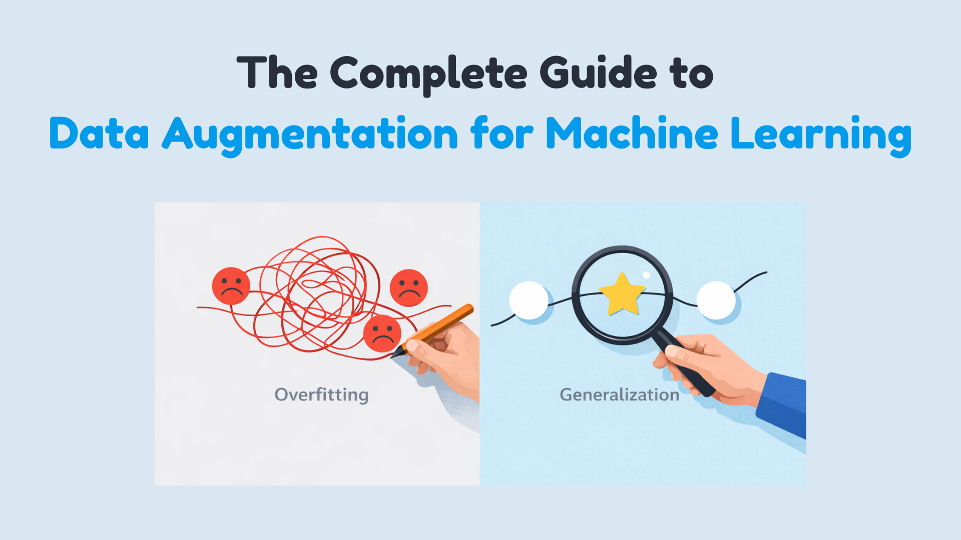
The Complete Guide to Data Augmentation for Machine Learning
In this article, you will learn practical, safe ways to use data augmentation to reduce overfitting and improve generalization across images, text, audio, and tabular datasets. Topics we will cover include: How augmentation works and when it helps. Online vs. offline augmentation strategies. Hands-on examples for images (TensorFlow/Keras), text (NLTK), audio (librosa), and tabular data (NumPy/Pandas), plus the critical pitfalls of data leakage. Alright, let’s get to it. The Complete Guide to Data Augmentation for Machine LearningImage by Author Suppose you’ve built your machine learning model, run the experiments, and stared at the results wondering what went wrong. Training accuracy looks great, maybe even impressive, but when you check validation accuracy… not so much. You can solve this issue by getting more data. But that is slow, expensive, and sometimes just impossible. It’s not about inventing fake data. It’s about creating new training examples by subtly modifying the data you already have without changing its meaning or label. You’re showing your model the same concept in multiple forms. You are teaching what’s important and what can be ignored. Augmentation helps your model generalize instead of simply memorizing the training set. In this article, you’ll learn how data augmentation works in practice and when to use it. Specifically, we’ll cover: What data augmentation is and why it helps reduce overfitting The difference between offline and online data augmentation How to apply augmentation to image data with TensorFlow Simple and safe augmentation techniques for text data Common augmentation methods for audio and tabular datasets Why data leakage during augmentation can silently break your model Offline vs Online Data Augmentation Augmentation can happen before training or during training. Offline augmentation expands the dataset once and saves it. Online augmentation generates new variations every epoch. Deep learning pipelines usually prefer online augmentation because it exposes the model to effectively unbounded variation without increasing storage. Data Augmentation for Image Data Image data augmentation is the most intuitive place to start. A dog is still a dog if it’s slightly rotated, zoomed, or viewed under different lighting conditions. Your model needs to see these variations during training. Some common image augmentation techniques are: Rotation Flipping Resizing Cropping Zooming Shifting Shearing Brightness and contrast changes These transformations do not change the label—only the appearance. Let’s demonstrate with a simple example using TensorFlow and Keras: 1. Importing Libraries import tensorflow as tf from tensorflow.keras.datasets import mnist from tensorflow.keras.layers import Dense, Flatten, Conv2D, MaxPooling2D, Dropout from tensorflow.keras.utils import to_categorical from tensorflow.keras.preprocessing.image import ImageDataGenerator from tensorflow.keras.models import Sequential import tensorflow as tf from tensorflow.keras.datasets import mnist from tensorflow.keras.layers import Dense, Flatten, Conv2D, MaxPooling2D, Dropout from tensorflow.keras.utils import to_categorical from tensorflow.keras.preprocessing.image import ImageDataGenerator from tensorflow.keras.models import Sequential 2. Loading MNIST dataset (X_train, y_train), (X_test, y_test) = mnist.load_data() # Normalize pixel values X_train = X_train / 255.0 X_test = X_test / 255.0 # Reshape to (samples, height, width, channels) X_train = X_train.reshape(-1, 28, 28, 1) X_test = X_test.reshape(-1, 28, 28, 1) # One-hot encode labels y_train = to_categorical(y_train, 10) y_test = to_categorical(y_test, 10) (X_train, y_train), (X_test, y_test) = mnist.load_data() # Normalize pixel values X_train = X_train / 255.0 X_test = X_test / 255.0 # Reshape to (samples, height, width, channels) X_train = X_train.reshape(–1, 28, 28, 1) X_test = X_test.reshape(–1, 28, 28, 1) # One-hot encode labels y_train = to_categorical(y_train, 10) y_test = to_categorical(y_test, 10) Output: Downloading data from https://storage.googleapis.com/tensorflow/tf-keras-datasets/mnist.npz Downloading data from https://storage.googleapis.com/tensorflow/tf-keras-datasets/mnist.npz 3. Defining ImageDataGenerator for augmentation datagen = ImageDataGenerator( rotation_range=15, # rotate images by ±15 degrees width_shift_range=0.1, # 10% horizontal shift height_shift_range=0.1, # 10% vertical shift zoom_range=0.1, # zoom in/out by 10% shear_range=0.1, # apply shear transformation horizontal_flip=False, # not needed for digits fill_mode=”nearest” # fill missing pixels after transformations ) datagen = ImageDataGenerator( rotation_range=15, # rotate images by ±15 degrees width_shift_range=0.1, # 10% horizontal shift height_shift_range=0.1, # 10% vertical shift zoom_range=0.1, # zoom in/out by 10% shear_range=0.1, # apply shear transformation horizontal_flip=False, # not needed for digits fill_mode=‘nearest’ # fill missing pixels after transformations ) 4. Building a Simple CNN Model model = Sequential([ Conv2D(32, (3, 3), activation=’relu’, input_shape=(28, 28, 1)), MaxPooling2D((2, 2)), Conv2D(64, (3, 3), activation=’relu’), MaxPooling2D((2, 2)), Flatten(), Dropout(0.3), Dense(64, activation=’relu’), Dense(10, activation=’softmax’) ]) model.compile(optimizer=”adam”, loss=”categorical_crossentropy”, metrics=[‘accuracy’]) model = Sequential([ Conv2D(32, (3, 3), activation=‘relu’, input_shape=(28, 28, 1)), MaxPooling2D((2, 2)), Conv2D(64, (3, 3), activation=‘relu’), MaxPooling2D((2, 2)), Flatten(), Dropout(0.3), Dense(64, activation=‘relu’), Dense(10, activation=‘softmax’) ]) model.compile(optimizer=‘adam’, loss=‘categorical_crossentropy’, metrics=[‘accuracy’]) 5. Training the model batch_size = 64 epochs = 5 history = model.fit( datagen.flow(X_train, y_train, batch_size=batch_size, shuffle=True), steps_per_epoch=len(X_train)//batch_size, epochs=epochs, validation_data=(X_test, y_test) ) batch_size = 64 epochs = 5 history = model.fit( datagen.flow(X_train, y_train, batch_size=batch_size, shuffle=True), steps_per_epoch=len(X_train)//batch_size, epochs=epochs, validation_data=(X_test, y_test) ) Output: 6. Visualizing Augmented Images import matplotlib.pyplot as plt # Visualize five augmented variants of the first training sample plt.figure(figsize=(10, 2)) for i, batch in enumerate(datagen.flow(X_train[:1], batch_size=1)): plt.subplot(1, 5, i + 1) plt.imshow(batch[0].reshape(28, 28), cmap=’gray’) plt.axis(‘off’) if i == 4: break plt.show() import matplotlib.pyplot as plt # Visualize five augmented variants of the first training sample plt.figure(figsize=(10, 2)) for i, batch in enumerate(datagen.flow(X_train[:1], batch_size=1)): plt.subplot(1, 5, i + 1) plt.imshow(batch[0].reshape(28, 28), cmap=‘gray’) plt.axis(‘off’) if i == 4: break plt.show() Output: Data Augmentation for Textual Data Text is more delicate. You can’t randomly replace words without thinking about meaning. But small, controlled changes can help your model generalize. A simple example using synonym replacement (with NLTK): import nltk from nltk.corpus import wordnet import random nltk.download(“wordnet”) nltk.download(“omw-1.4”) def synonym_replacement(sentence): words = sentence.split() if not words: return sentence idx = random.randint(0, len(words) – 1) synsets = wordnet.synsets(words[idx]) if synsets and synsets[0].lemmas(): replacement = synsets[0].lemmas()[0].name().replace(“_”, ” “) words[idx] = replacement return ” “.join(words) text = “The movie was really good” print(synonym_replacement(text)) 1 2 3 4 5 6 7 8 9 10 11 12 13 14 15 16 17 18 19 20 import nltk from nltk.corpus import wordnet import random nltk.download(“wordnet”) nltk.download(“omw-1.4”) def synonym_replacement(sentence): words = sentence.split() if

Elon Musk Seeks Up To $134bn From OpenAI, Microsoft In Damages Over Fraudulent Partnership | Technology News
New Delhi: Tesla CEO and founder of AI firm xAI Elon Musk has asked a US federal court to award him $79 billion to $134 billion in damages, alleging that OpenAI and Microsoft defrauded him by abandoning OpenAI’s nonprofit mission and partnering with the software giant. Elon Musk’s lawyers filed the damages request a day after a judge denied OpenAI and Microsoft’s final bid to avoid a jury trial scheduled for late April in Oakland, California, according to multiple reports. The filing cited calculations that showed Musk is entitled to a share of OpenAI’s current $500 billion valuation as he donated $38 million in seed funding during the founding stage of the company in 2015. “Just as an early investor in a startup company may realise gains many orders of magnitude greater than the investor’s initial investment, the wrongful gains that OpenAI and Microsoft have earned — and which Musk is now entitled to disgorge — are much larger than Musk’s initial contributions,” the filing said. Add Zee News as a Preferred Source According to court papers, Musk’s side argued that $65.5 billion to $109.43 billions of alleged wrongful gains were made by OpenAI and $13.3 billion to $25.06 billion by Microsoft from Musk’s financial and non-monetary contributions, including technical and business advice. OpenAI and Microsoft have denied the allegations. Musk left OpenAI’s board in 2018, launched his own AI company in 2023, and sued OpenAI in 2024, challenging co-founder Sam Altman’s move to operate the company as a for‑profit entity. “Musk’s lawsuit continues to be baseless and a part of his ongoing pattern of harassment, and we look forward to demonstrating this at trial,” OpenAI said in a statement, adding, “this latest unserious demand is aimed solely at furthering this harassment campaign.” Meanwhile, Musk’s AI firm xAI is also suing Apple and OpenAI over an earlier integration of ChatGPT into Siri and Apple Intelligence as an optional add-on. Elon Musk alleged that Apple’s App Store practices disadvantage rivals such as Grok, and the lawsuit has survived initial dismissal.

Quantizing LLMs Step-by-Step: Converting FP16 Models to GGUF
In this article, you will learn how quantization shrinks large language models and how to convert an FP16 checkpoint into an efficient GGUF file you can share and run locally. Topics we will cover include: What precision types (FP32, FP16, 8-bit, 4-bit) mean for model size and speed How to use huggingface_hub to fetch a model and authenticate How to convert to GGUF with llama.cpp and upload the result to Hugging Face And away we go. Quantizing LLMs Step-by-Step: Converting FP16 Models to GGUFImage by Author Introduction Large language models like LLaMA, Mistral, and Qwen have billions of parameters that demand a lot of memory and compute power. For example, running LLaMA 7B in full precision can require over 12 GB of VRAM, making it impractical for many users. You can check the details in this Hugging Face discussion. Don’t worry about what “full precision” means yet; we’ll break it down soon. The main idea is this: these models are too big to run on standard hardware without help. Quantization is that help. Quantization allows independent researchers and hobbyists to run large models on personal computers by shrinking the size of the model without severely impacting performance. In this guide, we’ll explore how quantization works, what different precision formats mean, and then walk through quantizing a sample FP16 model into a GGUF format and uploading it to Hugging Face. What Is Quantization? At a very basic level, quantization is about making a model smaller without breaking it. Large language models are made up of billions of numerical values called weights. These numbers control how strongly different parts of the network influence each other when producing an output. By default, these weights are stored using high-precision formats such as FP32 or FP16, which means every number takes up a lot of memory, and when you have billions of them, things get out of hand very quickly. Take a single number like 2.31384. In FP32, that one number alone uses 32 bits of memory. Now imagine storing billions of numbers like that. This is why a 7B model can easily take around 28 GB in FP32 and about 14 GB even in FP16. For most laptops and GPUs, that’s already too much. Quantization fixes this by saying: we don’t actually need that much precision anymore. Instead of storing 2.31384 exactly, we store something close to it using fewer bits. Maybe it becomes 2.3 or a nearby integer value under the hood. The number is slightly less accurate, but the model still behaves the same in practice. Neural networks can tolerate these small errors because the final output depends on billions of calculations, not a single number. Small differences average out, much like image compression reduces file size without ruining how the image looks. But the payoff is huge. A model that needs 14 GB in FP16 can often run in about 7 GB with 8-bit quantization, or even around 4 GB with 4-bit quantization. This is what makes it possible to run large language models locally instead of relying on expensive servers. After quantizing, we often store the model in a unified file format. One popular format is GGUF, created by Georgi Gerganov (author of llama.cpp). GGUF is a single-file format that includes both the quantized weights and useful metadata. It’s optimized for quick loading and inference on CPUs or other lightweight runtimes. GGUF also supports multiple quantization types (like Q4_0, Q8_0) and works well on CPUs and low-end GPUs. Hopefully, this clarifies both the concept and the motivation behind quantization. Now let’s move on to writing some code. Step-by-Step: Quantizing a Model to GGUF 1. Installing Dependencies and Logging to Hugging Face Before downloading or converting any model, we need to install the required Python packages and authenticate with Hugging Face. We’ll use huggingface_hub, Transformers, and SentencePiece. This ensures we can access public or gated models without errors: !pip install -U huggingface_hub transformers sentencepiece -q from huggingface_hub import login login() !pip install –U huggingface_hub transformers sentencepiece –q from huggingface_hub import login login() 2. Downloading a Pre-trained Model We will pick a small FP16 model from Hugging Face. Here we use TinyLlama 1.1B, which is small enough to run in Colab but still gives a good demonstration. Using Python, we can download it with huggingface_hub: from huggingface_hub import snapshot_download model_id = “TinyLlama/TinyLlama-1.1B-Chat-v1.0″ snapshot_download( repo_id=model_id, local_dir=”model_folder”, local_dir_use_symlinks=False ) from huggingface_hub import snapshot_download model_id = “TinyLlama/TinyLlama-1.1B-Chat-v1.0” snapshot_download( repo_id=model_id, local_dir=“model_folder”, local_dir_use_symlinks=False ) This command saves the model files into the model_folder directory. You can replace model_id with any Hugging Face model ID that you want to quantize. (If needed, you can also use AutoModel.from_pretrained with torch.float16 to load it first, but snapshot_download is straightforward for grabbing the files.) 3. Setting Up the Conversion Tools Next, we clone the llama.cpp repository, which contains the conversion scripts. In Colab: !git clone https://github.com/ggml-org/llama.cpp !pip install -r llama.cpp/requirements.txt -q !git clone https://github.com/ggml-org/llama.cpp !pip install –r llama.cpp/requirements.txt –q This gives you access to convert_hf_to_gguf.py. The Python requirements ensure you have all needed libraries to run the script. 4. Converting the Model to GGUF with Quantization Now, run the conversion script, specifying the input folder, output filename, and quantization type. We will use q8_0 (8-bit quantization). This will roughly halve the memory footprint of the model: !python3 llama.cpp/convert_hf_to_gguf.py /content/model_folder \ –outfile /content/tinyllama-1.1b-chat.Q8_0.gguf \ –outtype q8_0 !python3 llama.cpp/convert_hf_to_gguf.py /content/model_folder \ —outfile /content/tinyllama–1.1b–chat.Q8_0.gguf \ —outtype q8_0 Here /content/model_folder is where we downloaded the model, /content/tinyllama-1.1b-chat.Q8_0.gguf is the output GGUF file, and the –outtype q8_0 flag means “quantize to 8-bit.” The script loads the FP16 weights, converts them into 8-bit values, and writes a single GGUF file. This file is now much smaller and ready for inference with GGUF-compatible tools. Output: INFO:gguf.gguf_writer:Writing the following files: INFO:gguf.gguf_writer:/content/tinyllama-1.1b-chat.Q8_0.gguf: n_tensors = 201, total_size = 1.2G Writing: 100% 1.17G/1.17G [00:26<00:00, 44.5Mbyte/s] INFO:hf-to-gguf:Model successfully exported to /content/tinyllama-1.1b-chat.Q8_0.gguf Output: INFO:gguf.gguf_writer:Writing the following files: INFO:gguf.gguf_writer:/content/tinyllama–1.1b–chat.Q8_0.gguf: n_tensors = 201, total_size = 1.2G Writing: 100% 1.17G/1.17G [00:26<00:00, 44.5Mbyte/s] INFO:hf–to–gguf:Model successfully exported to /content/tinyllama–1.1b–chat.Q8_0.gguf You can verify the output:
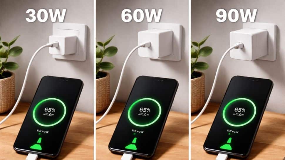
Worried About Your Smartphone’s Battery Health? Check Which Charger Is Best: 30W, 60W, Or 90W–Does Charging Speed Affect Battery Life? | Technology News
Smartphone Battery Health: With smartphones supporting fast charging, charger ratings like 30W, 65W, or 90W have become common factors in phone charging and battery health discussions. Users often argue which is best and think a higher-watt charger is always better, but watt simply refers to the amount of power a charger can deliver. In technical terms, a watt (W) is a unit of power that shows how much energy is transferred per second. In chargers, wattage is calculated by multiplying voltage (V) and current (A). Higher wattage usually means the charger can supply more power, which leads to faster charging–if the phone supports it. 30W vs 90W Chargers: What’s The Difference? Add Zee News as a Preferred Source A 30W charger is commonly used with mid-range and some flagship smartphones. It offers balanced charging speed and generates less heat. On the other hand, a 90W charger is designed for phones that support ultra-fast charging, usually premium models. These chargers can refill the battery much faster, sometimes reaching 50 percent in under 15 minutes. However, if a phone supports only 30W charging, using a 90W charger will not force extra power into the device. The phone will draw only the power it is designed to handle. (Also Read: Amazon Great Republic Day Sale 2026: From iPhone Air To OnePlus 15R; Check Top Deals On Budget-Friendly Smartphones) Does Higher Wattage Harm Battery? A common concern among most people is whether fast charging affects battery life. Lithium-ion batteries, used in smartphones, are sensitive to heat. Higher-watt charging can generate more heat, especially during the early stages of charging. Over time, repeated exposure to high temperatures can reduce battery health. However, modern smartphones are built with battery management systems that control power flow, temperature, and charging speed to prevent damage. Many phones slow down charging once the battery reaches around 80 percent to protect long-term battery life. Charging Speed vs Battery Health Faster charging is convenient and time-saving, but slower charging can be good for battery health. Using a lower-watt charger, such as 20W or 30W, produces less heat and may help maintain battery health over several years. However, use of fast chargers does not harm battery health if the device is well-designed. Smartphone manufacturers test batteries to handle fast charging within safe limits. Which Charger Should You Use? The best charger is the one recommended by the phone manufacturer only. Using a certified charger that matches your phone’s supported wattage ensures safe and efficient charging. For daily use, moderate-watt chargers are ideal, while high-watt chargers are useful when fast charging is needed.

10 Ways to Use Embeddings for Tabular ML Tasks
10 Ways to Use Embeddings for Tabular ML TasksImage by Editor Introduction Embeddings — vector-based numerical representations of typically unstructured data like text — have been primarily popularized in the field of natural language processing (NLP). But they are also a powerful tool to represent or supplement tabular data in other machine learning workflows. Examples not only apply to text data, but also to categories with a high level of diversity of latent semantic properties. This article uncovers 10 insightful uses of embeddings to leverage data at its fullest in a variety of machine learning tasks, models, or projects as a whole. Initial Setup: Some of the 10 strategies described below will be accompanied by brief illustrative code excerpts. An example toy dataset used in the examples is provided first, along with the most basic and commonplace imports needed in most of them. import pandas as pd import numpy as np # Example customer reviews’ toy dataset df = pd.DataFrame({ “user_id”: [101, 102, 103, 101, 104], “product”: [“Phone”, “Laptop”, “Tablet”, “Laptop”, “Phone”], “category”: [“Electronics”, “Electronics”, “Electronics”, “Electronics”, “Electronics”], “review”: [“great battery”, “fast performance”, “light weight”, “solid build quality”, “amazing camera”], “rating”: [5, 4, 4, 5, 5] }) import pandas as pd import numpy as np # Example customer reviews’ toy dataset df = pd.DataFrame({ “user_id”: [101, 102, 103, 101, 104], “product”: [“Phone”, “Laptop”, “Tablet”, “Laptop”, “Phone”], “category”: [“Electronics”, “Electronics”, “Electronics”, “Electronics”, “Electronics”], “review”: [“great battery”, “fast performance”, “light weight”, “solid build quality”, “amazing camera”], “rating”: [5, 4, 4, 5, 5] }) 1. Encoding Categorical Features With Embeddings This is a useful approach in applications like recommender systems. Rather than being handled numerically, high-cardinality categorical features, like user and product IDs, are best turned into vector representations. This approach has been widely applied and shown to effectively capture the semantic aspects and relationships among users and products. This practical example defines a couple of embedding layers as part of a neural network model that takes user and product descriptors and converts them into embeddings. from tensorflow.keras.layers import Input, Embedding, Flatten, Dense, Concatenate from tensorflow.keras.models import Model # Numeric and categorical user_input = Input(shape=(1,)) user_embed = Embedding(input_dim=500, output_dim=8)(user_input) user_vec = Flatten()(user_embed) prod_input = Input(shape=(1,)) prod_embed = Embedding(input_dim=50, output_dim=8)(prod_input) prod_vec = Flatten()(prod_embed) concat = Concatenate()([user_vec, prod_vec]) output = Dense(1)(concat) model = Model([user_input, prod_input], output) model.compile(“adam”, “mse”) 1 2 3 4 5 6 7 8 9 10 11 12 13 14 15 16 17 from tensorflow.keras.layers import Input, Embedding, Flatten, Dense, Concatenate from tensorflow.keras.models import Model # Numeric and categorical user_input = Input(shape=(1,)) user_embed = Embedding(input_dim=500, output_dim=8)(user_input) user_vec = Flatten()(user_embed) prod_input = Input(shape=(1,)) prod_embed = Embedding(input_dim=50, output_dim=8)(prod_input) prod_vec = Flatten()(prod_embed) concat = Concatenate()([user_vec, prod_vec]) output = Dense(1)(concat) model = Model([user_input, prod_input], output) model.compile(“adam”, “mse”) 2. Averaging Word Embeddings for Text Columns This approach compresses multiple texts of variable length into fixed-size embeddings by aggregating word-wise embeddings within each text sequence. It resembles one of the most common uses of embeddings; the twist here is aggregating word-level embeddings into a sentence- or text-level embedding. The following example uses Gensim, which implements the popular Word2Vec algorithm to turn linguistic units (typically words) into embeddings, and performs an aggregation of multiple word-level embeddings to create an embedding associated with each user review. from gensim.models import Word2Vec # Train embeddings on the review text sentences = df[“review”].str.lower().str.split().tolist() w2v = Word2Vec(sentences, vector_size=16, min_count=1) df[“review_emb”] = df[“review”].apply( lambda t: np.mean([w2v.wv[w] for w in t.lower().split()], axis=0) ) from gensim.models import Word2Vec # Train embeddings on the review text sentences = df[“review”].str.lower().str.split().tolist() w2v = Word2Vec(sentences, vector_size=16, min_count=1) df[“review_emb”] = df[“review”].apply( lambda t: np.mean([w2v.wv[w] for w in t.lower().split()], axis=0) ) 3. Clustering Embeddings Into Meta-Features Vertically stacking multiple individual embedding vectors into a 2D NumPy array (a matrix) is the core step to perform clustering on a set of customer review embeddings and identify natural groupings that might relate to topics in the review set. This technique captures coarse semantic clusters and can yield new, informative categorical features. from sklearn.cluster import KMeans emb_matrix = np.vstack(df[“review_emb”].values) km = KMeans(n_clusters=3, random_state=42).fit(emb_matrix) df[“review_topic”] = km.labels_ from sklearn.cluster import KMeans emb_matrix = np.vstack(df[“review_emb”].values) km = KMeans(n_clusters=3, random_state=42).fit(emb_matrix) df[“review_topic”] = km.labels_ 4. Learning Self-Supervised Tabular Embeddings As surprising as it may sound, learning numerical vector representations of structured data — particularly for unlabeled datasets — is a clever way to turn an unsupervised problem into a self-supervised learning problem: the data itself generates training signals. While these approaches are a bit more elaborate than the practical scope of this article, they commonly use one of the following strategies: Masked feature prediction: randomly hide some features’ values — similar to masked language modeling for training large language models (LLMs) — forcing the model to predict them based on the remaining visible features. Perturbation detection: expose the model to a noisy variant of the data, with some feature values swapped or replaced, and set the training goal as identifying which values are “legitimate” and which ones have been altered. 5. Building Multi-Labeled Categorical Embeddings This is a robust approach to prevent runtime errors when certain categories are not in the vocabulary used by embedding algorithms like Word2Vec, while maintaining the usability of embeddings. This example represents a single category like “Phone” using multiple tags such as “mobile” or “touch.” It builds a composite semantic embedding by aggregating the embeddings of associated tags. Compared to standard categorical encodings like one-hot, this method captures similarity more accurately and leverages knowledge beyond what Word2Vec “knows.” tags = { “Phone”: [“mobile”, “touch”], “Laptop”: [“portable”, “cpu”], “Tablet”: [] # Added to handle the ‘Tablet’ product } def safe_mean_embedding(words, model, dim): vecs = [model.wv[w] for w in words if w in model.wv] return np.mean(vecs, axis=0) if vecs else np.zeros(dim) df[“tag_emb”] = df[“product”].apply( lambda p: safe_mean_embedding(tags[p], w2v, 16) ) tags = { “Phone”: [“mobile”, “touch”], “Laptop”: [“portable”, “cpu”], “Tablet”: [] # Added to handle the ‘Tablet’ product } def safe_mean_embedding(words, model, dim): vecs = [model.wv[w] for w in

YouTube Earnings In India: How Much Creators Earn Per 1,000 Views, Top Creator Secrets, And Monetization Rules Revealed | Technology News
YouTube Earnings Per 1000 Views In India: YouTube is often seen as a platform for entertainment and time pass. However, behind popular videos, many creators are building successful careers. In India, several YouTubers earn crores of rupees by creating content that attracts large and loyal audiences. Their success does not come overnight. It starts with regular uploads and a clear understanding of what viewers want to watch. Creators working in gaming, comedy, tech, and education slowly grow their reach. Over time, they earn not only through advertisements but also through brand deals and their own products, which becomes the real source of massive income. In this article, we explain what they do to make their videos reach millions of views so that you can also run your YouTube channel in a similar way and earn crores. What are YouTube earnings per 1,000 views in India? Add Zee News as a Preferred Source YouTube Earnings Start With Google AdSense For most creators, YouTube earnings start with Google AdSense. As videos get more views and watch time increases, ad revenue grows. But successful creators know that AdSense is only the beginning. They treat it as a foundation while exploring other ways to scale their income. YouTube Earnings: Brand Deals And Sponsorships The real money for top YouTubers comes from brand deals and sponsorships. Channels with a loyal and engaged audience attract brands willing to pay anywhere from lakhs to crores for a single video. In this case, audience trust and quality matter more than just follower count. YouTube Earnings: Personal Brand By Selling Online Courses Top YouTubers do more than just make videos. They build a personal brand by selling online courses, e-books, or merchandise. The trust they earn from their audience turns these ventures into steady income and helps them expand beyond YouTube, ensuring long-term success. YouTube Earnings: Affiliate Marketing Affiliate marketing has become a key income source for many creators. They place product links in video descriptions or comments and earn a commission whenever viewers make a purchase. This method is particularly effective in niches such as tech, beauty, fitness, and education, allowing creators to earn consistently while providing their audience with useful products and recommendations. YouTube Earnings: Secret Formula To Make Crores Successful creators do not just follow trends, they set them. They have a strong understanding of SEO, thumbnails, titles, and audience behavior. Regular uploads, consistent timing, and content that provides real value are their most powerful tools. These strategies help them stand out on a crowded platform. In conclusion, there is no shortcut to earning crores on YouTube. With the right planning and approach, it is possible. Creators who treat YouTube as a business focus on trust and value, not just views, and that is what drives long-term success. YouTube Earnings Per 1000 Views In India In India, YouTube earnings per 1,000 views, called RPM, usually range from Rs 50 to Rs 200 after YouTube takes its 45% share. Earnings depend on the niche, audience location, ad engagement, and video length. Finance or tech videos often earn more, around Rs 100 to 300 per 1,000 views. Not all views generate money because only views with ads count, and views from foreign audiences can increase earnings. YouTube Monetization Rules To earn money on YouTube, a channel must meet basic eligibility requirements. It needs at least 1,000 subscribers and either 4,000 valid public watch hours in the past 12 months or 10 million valid views on Shorts within the last 90 days. Meeting these thresholds allows creators to apply for monetization and start earning revenue from their content.

How to Read a Machine Learning Research Paper in 2026
In this article, you will learn a practical, question-driven workflow for reading machine learning research papers efficiently, so you finish with answers — not fatigue. Topics we will cover include: Why purpose-first reading beats linear, start-to-finish reading. A lightweight triage: title + abstract + five-minute skim. How to target sections to answer your questions and retain what matters. Let’s not waste any more time. How to Read a Machine Learning Research Paper in 2026Image by Author Introduction When I first started reading machine learning research papers, I honestly thought something was wrong with me. I would open a paper, read the first few pages carefully, and then slowly lose focus. By the time I reached the middle, I felt tired, confused, and unsure what I had actually learned. During literature reviews, this feeling became even worse. Reading multiple long papers in a row drained my energy, and I often felt frustrated instead of confident. At first, I assumed this was just my lack of experience. But after talking to others in my research community, I realized this struggle is extremely common. Many beginners feel overwhelmed when reading papers, especially in machine learning where ideas, terminology, and assumptions move fast. Over time, and after spending more than two years around research, I realized the issue was not me. The issue was how I was reading papers. One Idea That Changed Everything for Me Most beginners approach research papers the same way they approach textbooks or articles: start from the beginning and read until the end. The problem is that research papers are not written to be read that way. They are written for people who already have questions in mind. If you read without knowing what you are looking for, your brain has no anchor. That is why everything starts to blur together after a few pages. Once I understood this, my entire approach changed. The biggest shift I made was simple: Never read a paper without a reason. A paper is not something you read just to finish it. You read it to answer questions. If you do not have questions, the paper will feel meaningless and exhausting. This idea really clicked for me after taking a course on Adaptive AI by Evan Shelhamer (formerly at Google DeepMind). I will not get into who originally proposed the technique, but the mindset behind it completely changed how I read papers. Since then, reading papers has felt lighter and much more manageable. And I will share the strategy in this article. Starting With Only the Title and Abstract Whenever I open a new paper now, I do not jump into the introduction. I only read two things: The title The abstract I spend no more than one or two minutes here. At this point, I am only trying to understand three things in a very rough way: What problem is this paper trying to solve? What kind of solution are they proposing? Do I care about this problem right now? If the answer to the last question is no, I skip the paper. And that is completely okay. You do not need to read every paper you open. Writing Down What Confuses You After reading the abstract, I stop. Before reading anything else, I write down what I did not understand or what made me curious. This step sounds small, but it makes a huge difference. For example, when I read the abstract of the paper “Test-Time Training with Self-Supervision for Generalization under Distribution Shifts”, I was confused at one point and wrote this question in my notes. What exactly do they mean by “turning a single unlabeled test sample into a self-supervised learning problem”? I knew what self-supervised learning was, but I could not picture how that would work for the problem being discussed in the paper. So I wrote that question down. That question gave me a reason to continue reading. I was no longer reading blindly. I was reading to find an answer. If you understand the problem statement reasonably well, pause for a moment and ask yourself: How would I approach this problem? What naive or baseline solution would I try? What assumptions would I make? This part is optional, but it helps you actively compare your thinking with the authors’ decisions. Doing a Quick Skim Instead of Deep Reading Once I have my questions, I do a quick skim of the paper. This usually takes around five minutes. I do not read every line. Instead, I focus on: The introduction, to see how the authors explain the problem—only if I am not aware of the background knowledge of that paper. Figures and diagrams, because they often explain more than text. A high-level look at the method section, just to see what is happening overall. The results, to understand what actually improved. At this stage, I am not trying to fully understand the method. I am just building a rough picture. Asking Better Questions After skimming, I usually end up with more questions than I started with. And that is a good thing. These questions are more specific now. They might be about why certain design choices were made, why some results look better than others, or what assumptions the method relies on. This is the point where reading starts to feel interesting instead of exhausting. Reading Only What Helps Answer Your Questions Now I finally read more carefully, but still not from start to end. I jump to the parts of the paper that help answer my questions. I search for keywords using Ctrl + F / Cmd + F, check the appendix, and sometimes skim related work that the authors say they are closely building on. My goal is not to understand everything. My goal is to understand what I care about. By the time I reach the end, I usually feel satisfied instead of tired, because my questions have been answered. I also start to see gaps, limitations, and opportunities much more clearly, because

iQOO Z11 Turbo Launched With 7,600mAh Battery, 100W Fast Charging, And More – Check Price, Colours, Variants | Technology News
iQOO Z11 Turbo: The Chinese smartphone maker iQOO has launched the iQOO Z11 Turbo in China as the latest addition to its Z-series lineup. The device was introduced on Thursday and is now available for purchase through the Vivo online store in the country. The phone comes in four colour options and multiple RAM and storage variants. The iQOO Z11 Turbo is offered in five configurations and colour options include Polar Night Black, Skylight White, Canglang Fuguang, and Halo Powder. Variant (RAM + Storage) wise expected prices are listed below: Add Zee News as a Preferred Source 12GB + 256GB CNY 2,699 at Rs 35,999 16GB + 256GB CNY 2,999 at Rs 39,000 12GB + 512GB CNY 3,199 at Rs 41,000 16GB + 512GB CNY 3,499 at Rs 45,000 16GB + 1TB CNY 3,999 at Rs 52,000 The smartphone features a 6.59-inch amoled display with 1.5K resolution and a 144Hz refresh rate. It supports HDR content and offers a high screen-to-body ratio of over 94 percent. The phone runs on Android 16-based OriginOS 6 and supports dual SIM functionality. iQOO has also confirmed IP68 and IP69 ratings, making the device resistant to dust and water.

No More Use Of ChatGPT On WhatsApp: Meta’s New Rules End Access For 50M Users – Check How To Save Your Chat History | Technology News
OpenAI’s popular AI chatbot, ChatGPT, can no longer be used on WhatsApp starting today, January 15, 2026. This change comes after Meta, WhatsApp’s parent company, updated its business API policies to restrict general-purpose AI chatbots like ChatGPT. Over 50 million users who enjoyed chatting, creating, and learning via WhatsApp now won’t be able to use ChatGPT on WhatsApp. In October 2025, Meta introduced new rules to limit AI companies from using WhatsApp as a main hub for broad AI assistants. The policy blocks services that run open-ended conversations or share user data for AI training. OpenAI confirmed the end of support, saying they preferred to stay but must follow the terms. This affects text chats and calls to the number +1 (800) 242-8478. Users in India and worldwide will experience this OpenAI update, as WhatsApp has billions of active users. Many relied on ChatGPT for quick answers, image generation, and web searches right in their chats. Add Zee News as a Preferred Source (Also Read: BGMI 4.2 Update Release Date & Time: Primewood Genesis Theme, Royal Enfield Bikes, New Modes, Abilities, And More – Check How To Download) How To Save Your Chat History? OpenAI has urged users to act fast to keep their conversations. Visit the ChatGPT contact profile in WhatsApp and click the link to connect your account. This links your phone number to ChatGPT and moves past chats to the official app. WhatsApp does not allow direct exports, so this is the only way before access cuts off completely. After linking, users can unlink their number if they want. However, ChatGPT is free and easy to use on Android, iOS apps, desktop, and web. OpenAI also launched its Atlas browser for Mac, with more platforms coming. Paid users get extra tools like agent mode for tasks such as research or tab cleanup.