
Access Denied You don’t have permission to access “http://zeenews.india.com/technology/india-replaces-china-in-us-smartphone-supply-chain-captures-40-share-report-3038361.html” on this server. Reference #18.c4f43717.1776433576.da13413a https://errors.edgesuite.net/18.c4f43717.1776433576.da13413a
Access Denied
Access Denied You don’t have permission to access “http://zeenews.india.com/technology/vivo-x300-ultra-x300-fe-india-launch-confirmed-check-expected-price-specs-features-3038452.html” on this server. Reference #18.c4f43717.1776428002.d93af4fb https://errors.edgesuite.net/18.c4f43717.1776428002.d93af4fb

Python Decorators for Production Machine Learning Engineering
In this article, you will learn how to use Python decorators to improve the reliability, observability, and efficiency of machine learning systems in production. Topics we will cover include: Implementing retry logic with exponential backoff for unstable external dependencies. Validating inputs and enforcing schemas before model inference. Optimizing performance with caching, memory guards, and monitoring decorators. Python Decorators for Production ML EngineeringImage by Editor Introduction You’ve probably written a decorator or two in your Python career. Maybe a simple @timer to benchmark a function, or a @login_required borrowed from Flask. But decorators become a completely different animal once you’re running machine learning models in production. Suddenly, you’re dealing with flaky API calls, memory leaks from massive tensors, input data that drifts without warning, and functions that need to fail gracefully at 3 AM when nobody’s watching. The five decorators in this article aren’t textbook examples. They’re patterns that solve real, recurring headaches in production machine learning systems, and they will change how you think about writing resilient inference code. 1. Automatic Retry with Exponential Backoff Production machine learning pipelines constantly interact with external services. You might be calling a model endpoint, pulling embeddings from a vector database, or fetching features from a remote store. These calls fail. Networks hiccup, services throttle requests, and cold starts introduce latency spikes. Wrapping every call in try/except blocks with retry logic quickly turns your codebase into a mess. Fortunately, @retry solves this elegantly. You define the decorator to accept parameters such as max_retries, backoff_factor, and a tuple of retriable exceptions. Inside, the wrapper function catches those specific exceptions, waits using exponential backoff (multiplying the delay after each attempt), and re-raises the exception if all retries are exhausted. The advantage here is that your core function remains clean. It simply performs the call. The resilience logic is centralized, and you can tune retry behavior per function through decorator arguments. For model-serving endpoints that occasionally experience timeouts, this single decorator can mean the difference between noisy alerts and seamless recovery. 2. Input Validation and Schema Enforcement Data quality issues are a silent failure mode in machine learning systems. Models are trained on features with specific distributions, types, and ranges. In production, upstream changes can introduce null values, incorrect data types, or unexpected shapes. By the time you detect the issue, your system may have been serving poor predictions for hours. A @validate_input decorator intercepts function arguments before they reach your model logic. You can design it to check whether a NumPy array matches an expected shape, whether required dictionary keys are present, or whether values fall within acceptable ranges. When validation fails, the decorator raises a descriptive error or returns a safe default response instead of allowing corrupted data to propagate downstream. This pattern pairs well with Pydantic if you want more sophisticated validation. However, even a lightweight implementation that checks array shapes and data types before inference will prevent many common production issues. It is a proactive defense rather than reactive debugging. 3. Result Caching with TTL If you are serving predictions in real time, you will encounter repeated inputs. For example, the same user may hit a recommendation endpoint multiple times in a session, or a batch job may reprocess overlapping feature sets. Running inference repeatedly wastes compute resources and adds unnecessary latency. A @cache_result decorator with a time-to-live (TTL) parameter stores function outputs keyed by their inputs. Internally, you maintain a dictionary mapping hashed arguments to tuples of (result, timestamp). Before executing the function, the wrapper checks whether a valid cached result exists. If the entry is still within the TTL window, it returns the cached value. Otherwise, it executes the function and updates the cache. The TTL component makes this approach production-ready. Predictions can become stale, especially when underlying features change. You want caching, but with an expiration policy that reflects how quickly your data evolves. In many real-time scenarios, even a short TTL of 30 seconds can significantly reduce redundant computation. 4. Memory-Aware Execution Large models consume significant memory. When running multiple models or processing large batches, it is easy to exceed available RAM and crash your service. These failures are often intermittent, depending on workload variability and garbage collection timing. A @memory_guard decorator checks available system memory before executing a function. Using psutil, it reads current memory usage and compares it against a configurable threshold (for example, 85% utilization). If memory is constrained, the decorator can trigger garbage collection with gc.collect(), log a warning, delay execution, or raise a custom exception that an orchestration layer can handle gracefully. This is especially useful in containerized environments, where memory limits are strict. Platforms such as Kubernetes will terminate your service if it exceeds its memory allocation. A memory guard gives your application an opportunity to degrade gracefully or recover before reaching that point. 5. Execution Logging and Monitoring Observability in machine learning systems extends beyond HTTP status codes. You need visibility into inference latency, anomalous inputs, shifting prediction distributions, and performance bottlenecks. While ad hoc logging works initially, it becomes inconsistent and difficult to maintain as systems grow. A @monitor decorator wraps functions with structured logging that captures execution time, input summaries, output characteristics, and exception details automatically. It can integrate with logging frameworks, Prometheus metrics, or observability platforms such as Datadog. The decorator timestamps execution start and end, logs exceptions before re-raising them, and optionally pushes metrics to a monitoring backend. The real value emerges when this decorator is applied consistently across the inference pipeline. You gain a unified, searchable record of predictions, execution times, and failures. When issues arise, engineers have actionable context instead of limited diagnostic information. Final Thoughts These five decorators share a common philosophy: keep core machine learning logic clean while pushing operational concerns to the edges. Decorators provide a natural separation that improves readability, testability, and maintainability. Start with the decorator that addresses your most immediate challenge. For many teams, that is retry logic or monitoring. Once you experience the clarity this pattern brings, it
Access Denied
Access Denied You don’t have permission to access “http://zeenews.india.com/technology/motorola-edge-70-pro-india-launch-set-for-april-22-key-features-specs-and-what-to-expect-3037954.html” on this server. Reference #18.eff43717.1776324035.98e6d81f https://errors.edgesuite.net/18.eff43717.1776324035.98e6d81f
Access Denied
Access Denied You don’t have permission to access “http://zeenews.india.com/technology/what-is-google-chrome-s-new-skills-feature-uses-benefits-and-how-it-helps-users-3037582.html” on this server. Reference #18.eff43717.1776274634.966ca72c https://errors.edgesuite.net/18.eff43717.1776274634.966ca72c
Access Denied
Access Denied You don’t have permission to access “http://zeenews.india.com/technology/is-your-laptop-slow-and-lagging-here-are-5-simple-tips-to-improve-its-performance-3037824.html” on this server. Reference #18.eff43717.1776268696.944cdace https://errors.edgesuite.net/18.eff43717.1776268696.944cdace
Access Denied
Access Denied You don’t have permission to access “http://zeenews.india.com/technology/india-ranks-among-world-s-most-advanced-ai-markets-openai-3037839.html” on this server. Reference #18.c4f43717.1776261498.bf089bad https://errors.edgesuite.net/18.c4f43717.1776261498.bf089bad
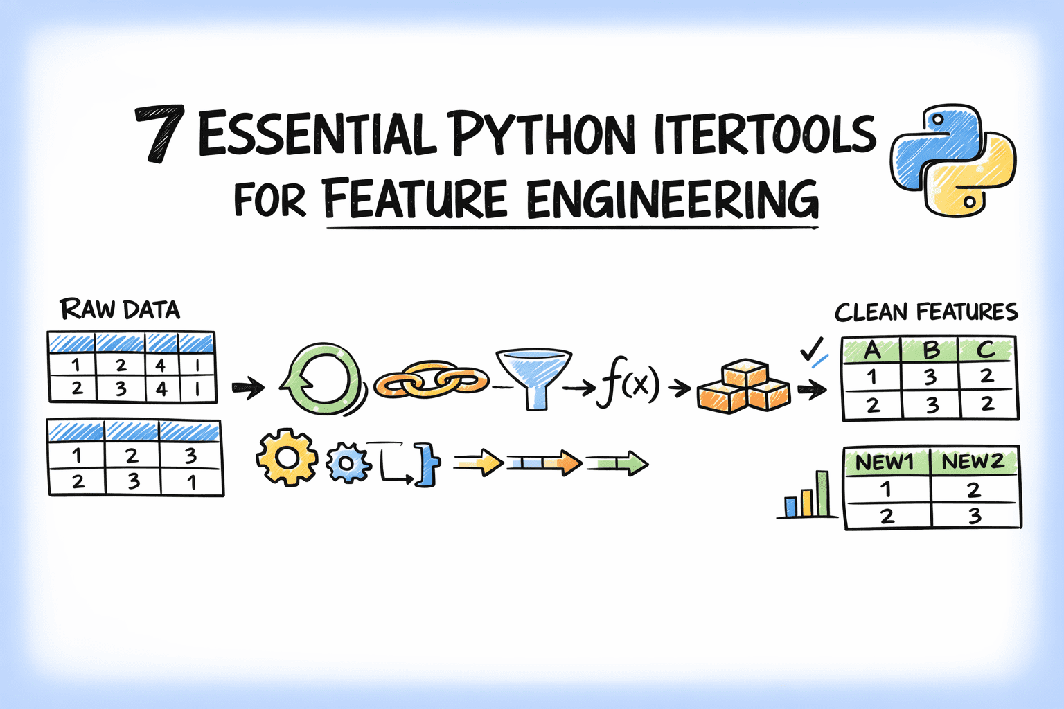
7 Essential Python Itertools for Feature Engineering
In this article, you will learn how to use Python’s itertools module to simplify common feature engineering tasks with clean, efficient patterns. Topics we will cover include: Generating interaction, polynomial, and cumulative features with itertools. Building lookup grids, lag windows, and grouped aggregates for structured data workflows. Using iterator-based tools to write cleaner, more composable feature engineering code. On we go. 7 Essential Python Itertools for Feature EngineeringImage by Editor Introduction Feature engineering is where most of the real work in machine learning happens. A good feature often improves a model more than switching algorithms. Yet this step usually leads to messy code with nested loops, manual indexing, hand-built combinations, and the like. Python’s itertools module is a standard library toolkit that most data scientists know exists but rarely reach for when building features. That’s a missed opportunity, as itertools is designed for working with iterators efficiently. A lot of feature engineering, at its core, is structured iteration over pairs of variables, sliding windows, grouped sequences, or every possible subset of a feature set. In this article, you’ll work through seven itertools functions that solve common feature engineering problems. We’ll spin up sample e-commerce data and cover interaction features, lag windows, category combinations, and more. By the end, you’ll have a set of patterns you can drop directly into your own feature engineering pipelines. You can get the code on GitHub. 1. Generating Interaction Features with combinations Interaction features capture the relationship between two variables — something neither variable expresses alone. Manually listing every pair from a multi-column dataset is tedious. combinations in the itertools module does it in one line. Let’s code an example to create interaction features using combinations: import itertools import pandas as pd df = pd.DataFrame({ “avg_order_value”: [142.5, 89.0, 210.3, 67.8, 185.0], “discount_rate”: [0.10, 0.25, 0.05, 0.30, 0.15], “days_since_signup”: [120, 45, 380, 12, 200], “items_per_order”: [3.2, 1.8, 5.1, 1.2, 4.0], “return_rate”: [0.05, 0.18, 0.02, 0.22, 0.08], }) numeric_cols = df.columns.tolist() for col_a, col_b in itertools.combinations(numeric_cols, 2): feature_name = f”{col_a}_x_{col_b}” df[feature_name] = df[col_a] * df[col_b] interaction_cols = [c for c in df.columns if “_x_” in c] print(df[interaction_cols].head()) 1 2 3 4 5 6 7 8 9 10 11 12 13 14 15 16 17 18 19 import itertools import pandas as pd df = pd.DataFrame({ “avg_order_value”: [142.5, 89.0, 210.3, 67.8, 185.0], “discount_rate”: [0.10, 0.25, 0.05, 0.30, 0.15], “days_since_signup”: [120, 45, 380, 12, 200], “items_per_order”: [3.2, 1.8, 5.1, 1.2, 4.0], “return_rate”: [0.05, 0.18, 0.02, 0.22, 0.08], }) numeric_cols = df.columns.tolist() for col_a, col_b in itertools.combinations(numeric_cols, 2): feature_name = f“{col_a}_x_{col_b}” df[feature_name] = df[col_a] * df[col_b] interaction_cols = [c for c in df.columns if “_x_” in c] print(df[interaction_cols].head()) Truncated output: avg_order_value_x_discount_rate avg_order_value_x_days_since_signup \ 0 14.250 17100.0 1 22.250 4005.0 2 10.515 79914.0 3 20.340 813.6 4 27.750 37000.0 avg_order_value_x_items_per_order avg_order_value_x_return_rate \ 0 456.00 7.125 1 160.20 16.020 2 1072.53 4.206 3 81.36 14.916 4 740.00 14.800 … days_since_signup_x_return_rate items_per_order_x_return_rate 0 6.00 0.160 1 8.10 0.324 2 7.60 0.102 3 2.64 0.264 4 16.00 0.320 1 2 3 4 5 6 7 8 9 10 11 12 13 14 15 16 17 18 19 20 21 avg_order_value_x_discount_rate avg_order_value_x_days_since_signup \ 0 14.250 17100.0 1 22.250 4005.0 2 10.515 79914.0 3 20.340 813.6 4 27.750 37000.0 avg_order_value_x_items_per_order avg_order_value_x_return_rate \ 0 456.00 7.125 1 160.20 16.020 2 1072.53 4.206 3 81.36 14.916 4 740.00 14.800 … days_since_signup_x_return_rate items_per_order_x_return_rate 0 6.00 0.160 1 8.10 0.324 2 7.60 0.102 3 2.64 0.264 4 16.00 0.320 combinations(numeric_cols, 2) generates every unique pair exactly once without duplicates. With 5 columns, that is 10 pairs; with 10 columns, it is 45. This approach scales as you add columns. 2. Building Cross-Category Feature Grids with product itertools.product gives you the Cartesian product of two or more iterables — every possible combination across them — including repeats across different groups. In the e-commerce sample we’re working with, this is useful when you want to build a feature matrix across customer segments and product categories. import itertools customer_segments = [“new”, “returning”, “vip”] product_categories = [“electronics”, “apparel”, “home_goods”, “beauty”] channels = [“mobile”, “desktop”] # All segment × category × channel combinations combos = list(itertools.product(customer_segments, product_categories, channels)) grid_df = pd.DataFrame(combos, columns=[“segment”, “category”, “channel”]) # Simulate a conversion rate lookup per combination import numpy as np np.random.seed(7) grid_df[“avg_conversion_rate”] = np.round( np.random.uniform(0.02, 0.18, size=len(grid_df)), 3 ) print(grid_df.head(12)) print(f”\nTotal combinations: {len(grid_df)}”) 1 2 3 4 5 6 7 8 9 10 11 12 13 14 15 16 17 18 19 20 import itertools customer_segments = [“new”, “returning”, “vip”] product_categories = [“electronics”, “apparel”, “home_goods”, “beauty”] channels = [“mobile”, “desktop”] # All segment × category × channel combinations combos = list(itertools.product(customer_segments, product_categories, channels)) grid_df = pd.DataFrame(combos, columns=[“segment”, “category”, “channel”]) # Simulate a conversion rate lookup per combination import numpy as np np.random.seed(7) grid_df[“avg_conversion_rate”] = np.round( np.random.uniform(0.02, 0.18, size=len(grid_df)), 3 ) print(grid_df.head(12)) print(f“\nTotal combinations: {len(grid_df)}”) Output: segment category channel avg_conversion_rate 0 new electronics mobile 0.032 1 new electronics desktop 0.145 2 new apparel mobile 0.090 3 new apparel desktop 0.136 4 new home_goods mobile 0.176 5 new home_goods desktop 0.106 6 new beauty mobile 0.100 7 new beauty desktop 0.032 8 returning electronics mobile 0.063 9 returning electronics desktop 0.100 10 returning apparel mobile 0.129 11 returning apparel desktop 0.149 Total combinations: 24 segment category channel avg_conversion_rate 0 new electronics mobile 0.032 1 new electronics desktop 0.145 2 new apparel mobile 0.090 3 new apparel desktop 0.136 4 new home_goods mobile 0.176 5 new home_goods desktop 0.106 6 new beauty mobile 0.100 7 new beauty desktop 0.032 8 returning electronics mobile 0.063 9 returning electronics desktop 0.100 10 returning apparel mobile 0.129 11 returning apparel desktop 0.149 Total combinations: 24 This grid can then be merged back onto your main transaction dataset as a lookup feature, as every row gets the expected conversion rate for its specific segment × category × channel bucket. product ensures you haven’t missed any valid combination when building that grid. 3. Flattening Multi-Source Feature Sets with chain In most pipelines, features come from multiple sources: a customer profile table, a product metadata table, and a browsing history table. You often need to flatten these into a single feature list for column selection
Access Denied
Access Denied You don’t have permission to access “http://zeenews.india.com/technology/vivo-t5-pro-5g-launched-in-india-at-rs-with-9020-mah-battery-check-camera-features-performance-and-variants-3037654.html” on this server. Reference #18.c4f43717.1776248107.bd0656a4 https://errors.edgesuite.net/18.c4f43717.1776248107.bd0656a4

From Prompt to Prediction: Understanding Prefill, Decode, and the KV Cache in LLMs
In the previous article, we saw how a language model converts logits into probabilities and samples the next token. But where do these logits come from? In this tutorial, we take a hands-on approach to understand the generation pipeline: How the prefill phase processes your entire prompt in a single parallel pass How the decode phase generates tokens one at a time using previously computed context How the KV cache eliminates redundant computation to make decoding efficient By the end, you will understand the two-phase mechanics behind LLM inference and why the KV cache is essential for generating long responses at scale. Let’s get started. From Prompt to Prediction: Understanding Prefill, Decode, and the KV Cache in LLMsPhoto by Neda Astani. Some rights reserved. Overview This article is divided into three parts; they are: How Attention Works During Prefill The Decode Phase of LLM Inference KV Cache: How to Make Decode More Efficient How Attention Works During Prefill Consider the prompt: Today’s weather is so … As humans, we can infer the next token should be an adjective, because the last word “so” is a setup. We also know it probably describes weather, so words like “nice” or “warm” are more likely than something unrelated like “delicious“. Transformers arrive at the same conclusion through attention. During prefill, the model processes the entire prompt in a single forward pass. Every token attends to itself and all tokens before it, building up a contextual representation that captures relationships across the full sequence. The mechanism behind this is the scaled dot-product attention formula: $$\text{Attention}(Q, K, V) = \mathrm{softmax}\left(\frac{QK^\top}{\sqrt{d_k}}\right)V$$ We will walk through this concretely below. To make the attention computation traceable, we assign each token a scalar value representing the information it carries: Position Tokens Values 1 Today 10 2 weather 20 3 is 1 4 so 5 Words like “is” and “so” carry less semantic weight than “Today” or “weather“, and as we’ll see, attention naturally reflects this. Attention Heads In real transformers, attention weights are continuous values learned during training through the $Q$ and $K$ dot product. The behavior of attention heads are learned and usually impossible to describe. No head is hardwired to “attend to even positions”. The four rules below are simplified illustration to make attention mechanism more intuitive, while the weighted aggregation over $V$ is the same. Here are the rules in our toy example: Attend to tokens at even number positions Attend to the last token Attend to the first token Attend to every token For simplicity in this example, the outputs from these heads are then combined (averaged). Let’s walk through the prefill process: Today Even tokens → none Last token → Today → 10 First token → Today → 10 All tokens → Today → 10 weather Even tokens → weather → 20 Last token → weather → 20 First token → Today → 10 All tokens → average(Today, weather) → 15 is Even tokens → weather → 20 Last token → is → 1 First token → Today → 10 All tokens → average(Today, weather, is) → 10.33 so Even tokens → average(weather, so) → 12.5 Last token → so → 5 First token → Today → 10 All tokens → average(Today, weather, is, so) → 9 Parallelizing Attention If the prompt contained 100,000 tokens, computing attention step-by-step would be extremely slow. Fortunately, attention can be expressed as tensor operations, allowing all positions to be computed in parallel. This is the key idea of prefill phase in LLM inference: When you provide a prompt, there are multiple tokens in it and they can be processed in parallel. Such parallel processing helps speed up the response time for the first token generated. To prevent tokens from seeing future tokens, we apply a causal mask, so they can only attend to itself and earlier tokens. import torch tokens = [“Today”, “weather”, “is”, “so”] n = len(tokens) d_k = 64 V = torch.tensor([[10.], [20.], [1.], [5.]], dtype=torch.float32) positions = torch.arange(1, n + 1).float() # 1-based: [1, 2, 3, 4] idx = torch.arange(n) causal_mask = idx.unsqueeze(1) >= idx.unsqueeze(0) print(causal_mask) import torch tokens = [“Today”, “weather”, “is”, “so”] n = len(tokens) d_k = 64 V = torch.tensor([[10.], [20.], [1.], [5.]], dtype=torch.float32) positions = torch.arange(1, n + 1).float() # 1-based: [1, 2, 3, 4] idx = torch.arange(n) causal_mask = idx.unsqueeze(1) >= idx.unsqueeze(0) print(causal_mask) Output: tensor([[ True, False, False, False], [ True, True, False, False], [ True, True, True, False], [ True, True, True, True]]) tensor([[ True, False, False, False], [ True, True, False, False], [ True, True, True, False], [ True, True, True, True]]) Now, we can start writing the “rules” for the 4 attention heads. Rather than computing scores from learned $Q$ and $K$ vectors, we handcraft them directly to match our four attention rules. Each head produces a score matrix of shape (n, n), with one score per query-key pair, which gets masked and passed through softmax to produce attention weights: def selector(condition, size): “””Return a (size, d_k) tensor of +1/-1 depending on condition.””” val = torch.where(condition, torch.ones( size), -torch.ones(size)) # (size,) # (size, d_k) return val.unsqueeze(1).expand(size, d_k).contiguous() # Shared query: every row asks for a property, and K encodes which tokens match it. Q = torch.ones(n, d_k) # Head 1: select even positions # K says whether each token is at an even position. K1 = selector(positions % 2 == 0, n) scores1 = (Q @ K1.T) / (d_k ** 0.5) # Head 2: select the last token # K says whether each token is the last one. K2 = selector(positions == n, n) scores2 = (Q @ K2.T) / (d_k ** 0.5) # Head 3: select the first token # K says whether each token is the first one. K3 = selector(positions == 1, n) scores3 = (Q @ K3.T) / (d_k ** 0.5) # Head 4: select all visible tokens uniformly # K says all the tokens K4 = selector(positions == positions, n) scores4