Access Denied You don’t have permission to access “http://zeenews.india.com/technology/dark-mode-vs-light-mode-in-summer-which-saves-more-battery-and-what-s-better-for-your-smartphone-3052388.html” on this server. Reference #18.5cfdd417.1780445840.ba9efd https://errors.edgesuite.net/18.5cfdd417.1780445840.ba9efd
Access Denied
Access Denied You don’t have permission to access “http://zeenews.india.com/technology/hack-of-the-day-how-to-stop-smartphone-apps-from-secretly-tracking-your-location-all-day-3052178.html” on this server. Reference #18.eff43717.1780386864.34d0f14a https://errors.edgesuite.net/18.eff43717.1780386864.34d0f14a
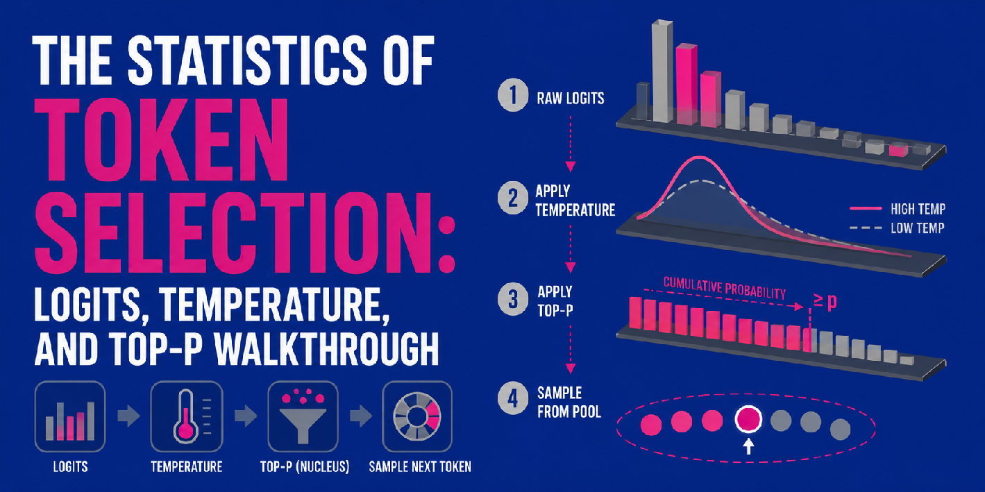
The Statistics of Token Selection: Logits, Temperature, and Top-P Walkthrough
In this article, you will learn how logits, temperature, and top-p sampling work together to control next-token prediction in large language models. Topics we will cover include: What logits are and how they are produced by a transformer’s final linear layer. How temperature and top-p (nucleus sampling) shape the probability distribution used for token selection. How these three components fit into a sequential pipeline that governs LLM output generation. The Statistics of Token Selection: Logits, Temperature, and Top-P Walkthrough Introduction When large language models, or LLMs for short, produce outputs, several criteria are at stake, including not only overall response relevance but also coherence and creativity. Since deep inside the models operate by building their response word by word — or more precisely, token by token — capturing these desirable properties is a matter of mathematically adjusting the output probability distributions that govern the next-token prediction process. This article introduces the mechanics behind LLM decoding strategies from a statistical vantage point. In particular, we will explore how raw model scores, known as logits, interact with two other model settings — temperature and top-p — which are three key parameters utilized to control the token selection process. While we will focus on exploring what happens inside the very final stages of the LLMs’ underlying architecture, a.k.a. the transformer, you can check this article if you need a concise overview of the whole process and journey made by tokens from beginning to end. Token selection process in LLMs What Are Logits? In neural networks, the raw, unnormalized scores produced (typically at final linear layers) before converting them into probabilities of possible outcomes (e.g. classes) are known as logits. While logits have been used since the era of classical machine learning classification models like softmax regression, the same principle still applies to the final linear layer of transformer models. This final layer processes hidden states — which contain gradually accumulated linguistic knowledge about the input text gathered throughout the transformer — and outputs a vector of logits. How many? As many as the model’s vocabulary size, i.e. the number of possible tokens the model can generate. See the diagram at the top, for instance. If an LLM trained for English-to-Spanish translation is predicting the next word after the generated sequence “me gusta mucho” (the translation of “I really like to”), it might output a raw logit score of 12.5 for “viajar” (travel), 8.2 for “jugar” (play), and -3.1 for “dormir” (sleep). These raw values are unbounded, making them difficult to interpret directly; hence, a softmax function is applied on top of the final linear layer to transform these logits into a standard, interpretable probability distribution over vocabulary tokens, such that all values sum to 1. What Are Temperature and Top-p? Once we have a probability distribution over the target vocabulary, do LLMs simply choose the token with the highest probability as the next one to generate? Not exactly, but the true process closely resembles that scenario. The next token is sampled from the distribution, and how this sampling works depends on several decoding parameters, two of the most important being temperature and top-p. Temperature is a scaling factor applied to the logits before the softmax step. A high temperature (e.g. above 1) flattens the resulting probabilities, making them more uniform. As a result, uncertainty and unpredictability increase, and the model behaves more creatively. A low temperature (e.g. well below 1) sharpens the differences between high- and low-probability tokens, increasing certainty and strongly favoring the most likely tokens in the original distribution. More about temperature can be found in this related article. Top-p, also called nucleus sampling, is another approach to controlling the randomness of next-token selection. Rather than scaling probabilities, it limits the pool of candidates to sample from. While similar strategies like top-k consider only the k highest-probability tokens, top-p identifies the smallest set of tokens whose cumulative probability meets or exceeds a threshold p, making it more adaptive and flexible. In other words, if we set p=0.9, top-p sorts tokens by probability and keeps adding them to a candidate pool until their cumulative probability reaches 0.9. The Full Walkthrough: How Do These Concepts Relate to Each Other? Logit-to-probability calculation, temperature, and top-p can be combined into a sequential multi-step pipeline for producing LLM outputs, i.e. next-token predictions. First, the model generates raw logits for all possible tokens, as described above. Temperature then enters the picture by scaling these raw logits — note that this happens before the softmax function converts them into probabilities. Depending on the temperature value, the resulting distribution will look more uniform (high temperature, more uncertainty) or sharper (low temperature, higher certainty). Token selection walkthrough based on logits, temperature, and top-p Once the scaled logits are converted into probabilities, top-p is applied to filter the resulting distribution, calculating cumulative probabilities to retain only a core “nucleus pool” of the most likely tokens (see step 3 in the image above). Finally, the model samples randomly from within that pool to select the next token. Closing Remarks Now that we have demystified the statistical process behind token selection in LLMs, it is useful to consider how to choose values for temperature and top-p in practice. As a developer, you will want to define the right balance between predictability and creativity for your use case. For factual, high-stakes scenarios like coding or legal analysis, a low temperature and a stricter top-p are advisable — e.g. t=0.1 and p=0.5 — which yields highly deterministic model responses. For creative domains like poetry generation or brainstorming, a higher temperature and top-p, such as t=0.8 and p=0.95, allow for a richer variety of candidate tokens in the selection pool.
Access Denied
Access Denied You don’t have permission to access “http://zeenews.india.com/technology/iphone-anti-snatch-auto-lock-whatsapp-blurred-spoiler-messages-3051714.html” on this server. Reference #18.c4f43717.1780235552.1132c70e https://errors.edgesuite.net/18.c4f43717.1780235552.1132c70e
Building a Context Pruning Pipeline for Long-Running Agents
In this article, you will learn how to implement a context pruning pipeline for long-running AI agents, enabling them to manage conversational memory efficiently through semantic similarity. Topics we will cover include: Why unbounded conversation history is a problem for agents built on top of large language models, and what a context pruning strategy looks like. How to use sentence transformer embedding models to compute semantic similarity between a current prompt and archived conversation turns. How to assemble a pruned context window from the most recent turn, the top-K semantically relevant past turns, and the current prompt. Building a Context Pruning Pipeline for Long-Running Agents Introduction Modern AI agents built on top of large language models (LLMs) are designed to run continuously. As a result, their conversation history keeps growing indefinitely. Passing such an entire history as the LLM’s context window is the perfect recipe for prohibitive token costs, latency bottlenecks, and eventual degradation in reasoning. Building a context pruning pipeline can address this issue by dynamically managing recent conversational memory. This article outlines the basic principles for implementing a context pruning pipeline for long-running agents. We use an entirely accessible and free-to-run local solution based on open-source embedding models rather than paid APIs, but you can replace them with paid APIs if you want a more efficient solution. Proposed Memory Strategy Classical memory strategies in agents rely on a sliding window that forgets old information as it falls behind, including potentially critical details. Moving beyond that approach, it is possible to build a selective, smarter pipeline that gives the LLM precisely what it needs as context. In essence, the context can be pruned down to the following basic elements: The current prompt, containing the user’s request or question. The most recent turn, i.e. the immediate previous input-response exchange, which is key to maintaining conversational continuity. The top-K semantically relevant matches, calculated based on a similarity score. These are past turns closely related to the current prompt, retrieved through vector embeddings. Everything in the conversation history that falls outside the scope of these three elements is discarded from the active prompt’s context, saving compute and memory. Simulation-Based Implementation Our example implementation simulates the application of the aforementioned strategy, building a context pruning window step by step. Sentence transformer models are used to simulate a long-running pipeline alongside a mocked conversation history. We start by making the necessary imports: import numpy as np from sentence_transformers import SentenceTransformer from scipy.spatial.distance import cosine import numpy as np from sentence_transformers import SentenceTransformer from scipy.spatial.distance import cosine Next, we load and initialize a pre-trained embedding model — concretely all-MiniLM-L6-v2 from the sentence_transformers library. This model has been trained to transform raw text into embedding vectors that capture semantic characteristics. We also create a simple, simulated agent history containing user-agent interactions (in a real setting, this would be fetched from a database): # Initialize a lightweight open-source embedding model model = SentenceTransformer(‘all-MiniLM-L6-v2’) # 1. Simulated Agent History (Usually fetched from a database) chat_history = [ {“role”: “user”, “content”: “My name is Alice and I work in logistics.”}, {“role”: “agent”, “content”: “Nice to meet you, Alice. How can I help with logistics?”}, {“role”: “user”, “content”: “What’s the weather like today?”}, {“role”: “agent”, “content”: “It’s sunny and 75 degrees.”}, {“role”: “user”, “content”: “I need help calculating route efficiency for my fleet.”}, {“role”: “agent”, “content”: “Route efficiency involves analyzing distance, traffic, and load weight.”}, {“role”: “user”, “content”: “Thanks, that makes sense.”}, {“role”: “agent”, “content”: “You’re welcome! Let me know if you need anything else.”} ] # Initialize a lightweight open-source embedding model model = SentenceTransformer(‘all-MiniLM-L6-v2’) # 1. Simulated Agent History (Usually fetched from a database) chat_history = [ {“role”: “user”, “content”: “My name is Alice and I work in logistics.”}, {“role”: “agent”, “content”: “Nice to meet you, Alice. How can I help with logistics?”}, {“role”: “user”, “content”: “What’s the weather like today?”}, {“role”: “agent”, “content”: “It’s sunny and 75 degrees.”}, {“role”: “user”, “content”: “I need help calculating route efficiency for my fleet.”}, {“role”: “agent”, “content”: “Route efficiency involves analyzing distance, traffic, and load weight.”}, {“role”: “user”, “content”: “Thanks, that makes sense.”}, {“role”: “agent”, “content”: “You’re welcome! Let me know if you need anything else.”} ] The core logic of the context pruning pipeline comes next. It is encapsulated in a prune_context() function that receives the current prompt, the full interaction history, and the number of semantically relevant past turns to retrieve, k: def prune_context(current_prompt, history, top_k=2): # If the conversation history is too short, we simply return it if len(history) <= 2: return history + [{“role”: “user”, “content”: current_prompt}] # Extracting the most recent turn (last user/agent pair) recent_turn = history[-2:] # The rest of the history will be eligible for semantic pruning archived_turns = history[:-2] # 2. Embedding the current prompt prompt_emb = model.encode(current_prompt) # 3. Embedding archived turns and computing similarities scored_turns = [] for turn in archived_turns: turn_emb = model.encode(turn[“content”]) # We want similarity, so we subtract cosine distance from 1 similarity = 1 – cosine(prompt_emb, turn_emb) scored_turns.append((similarity, turn)) # 4. Sorting by highest similarity and slicing the Top-K turns scored_turns.sort(key=lambda x: x[0], reverse=True) top_semantic_turns = [turn for score, turn in scored_turns[:top_k]] # Sorting the semantic turns chronologically (optional but recommended for LLMs) top_semantic_turns.sort(key=lambda x: archived_turns.index(x)) # 5. Assemble the final pruned context pruned_context = top_semantic_turns + recent_turn + [{“role”: “user”, “content”: current_prompt}] return pruned_context 1 2 3 4 5 6 7 8 9 10 11 12 13 14 15 16 17 18 19 20 21 22 23 24 25 26 27 28 29 30 31 32 33 def prune_context(current_prompt, history, top_k=2): # If the conversation history is too short, we simply return it if len(history) <= 2: return history + [{“role”: “user”, “content”: current_prompt}] # Extracting the most recent turn (last user/agent pair) recent_turn = history[–2:] # The rest of the history will be eligible for semantic pruning archived_turns = history[:–2] # 2. Embedding the current prompt prompt_emb = model.encode(current_prompt)
Access Denied
Access Denied You don’t have permission to access “http://zeenews.india.com/technology/hack-of-the-day-this-hidden-upi-setting-can-make-your-payments-safer-in-seconds-3051230.html” on this server. Reference #18.5cfdd417.1780089632.15e25ee3 https://errors.edgesuite.net/18.5cfdd417.1780089632.15e25ee3
Access Denied
Access Denied You don’t have permission to access “http://zeenews.india.com/technology/why-do-screenshots-reduce-image-quality-here-s-the-hidden-reason-behind-blurry-photos-solutions-inside-3051276.html” on this server. Reference #18.eff43717.1780070328.de79ca52 https://errors.edgesuite.net/18.eff43717.1780070328.de79ca52
Access Denied
Access Denied You don’t have permission to access “http://zeenews.india.com/technology/lava-bold-n2-5g-india-launch-set-for-june-3-heres-everything-you-need-to-know-3051380.html” on this server. Reference #18.3c0ec417.1780062384.51783144 https://errors.edgesuite.net/18.3c0ec417.1780062384.51783144
Access Denied
Access Denied You don’t have permission to access “http://zeenews.india.com/technology/whatsapp-instagram-facebook-premium-meta-s-new-paid-plan-to-offer-these-cool-features-subscription-cost-and-benefits-3051293.html” on this server. Reference #18.eff43717.1780044400.d65b7671 https://errors.edgesuite.net/18.eff43717.1780044400.d65b7671
Access Denied
Access Denied You don’t have permission to access “http://zeenews.india.com/technology/hack-of-the-day-this-hidden-whatsapp-privacy-feature-is-still-ignored-by-most-users-3050986.html” on this server. Reference #18.5cfdd417.1779955610.142672c8 https://errors.edgesuite.net/18.5cfdd417.1779955610.142672c8