
In this article, you will learn three practical strategies for managing small context windows in large language models, along with working Python examples that demonstrate how two of those strategies are implemented. Topics we will cover include: How context truncation via the sliding window approach keeps token usage flat and predictable. How token budgeting combined with retrieval-augmented generation ensures only the most relevant context fits within a prompt. A concise overview of additional strategies for more specialized use cases — rolling summaries, prompt compression, and observation masking. Introduction Top-tier AI industries have become somewhat obsessed with language models capable of ingesting massive context windows, e.g. an entire book in a single prompt. However, what they won’t admit easily is that in real-world LLM applications, these massive context windows come with various limitations and challenges, including soaring API costs, unacceptable response times, and even worse, the so-called “lost in the middle” problem whereby a model ignores data deeply buried in the middle of the giant prompt. No surprise, then, that working with small yet smartly managed context windows could yield superior outcomes, reducing latency, minimizing costs, and forcing the model to concentrate on what truly matters to generate its response. This article unveils three of the most widely adopted practical strategies for managing and mastering small context windows in language models, along with examples that mimic the implementation of some of them for better understanding. Context Truncation: Sliding Window There is a consensus that sliding windows are arguably the most common and simplest strategy for managing shortened context windows in language models. Instead of providing an entire user conversation history to the model, the context is treated as a FIFO (First-In-First-Out) queue: as new interactions (exchanged messages) come in, the oldest ones are simply dropped. All it takes is defining the size of the context window and striking a balance between sufficient past context retention and latency-cost control. The main advantage of truncating the context via sliding windows is absolute control and predictability over token usage and computing overhead. The maximum number of interactions dealt with by the model at a given time remains fixed, keeping latency flat and surprise-free. To better understand how this approach works, let’s look at the following Python code in which you can freely adjust the value of max_turns (context window size) and see how it affects the “memory” injected into the current prompt: class SlidingWindowMemory: def __init__(self, max_turns=3): “””Keep only the last `max_turns` of a conversation.””” self.max_turns = max_turns self.history = [] def add_interaction(self, user_text, ai_text): self.history.append({“user”: user_text, “ai”: ai_text}) # The logic behind a sliding window: drop the oldest turns if limits are surpassed if len(self.history) > self.max_turns: self.history = self.history[-self.max_turns:] def build_prompt(self, new_query): prompt = “System: Answer concisely based on recent context.\n\n” for turn in self.history: prompt += f”User: {turn[‘user’]}\nAI: {turn[‘ai’]}\n” prompt += f”User: {new_query}\nAI:” return prompt # — Testing the Sliding Window mechanism: feel free to adjust the value of max_turns — memory = SlidingWindowMemory(max_turns=2) # Simulating a long conversation memory.add_interaction(“Hi, I’m learning Python.”, “Great choice!”) memory.add_interaction(“What are lists?”, “Lists are mutable arrays.”) memory.add_interaction(“Can they hold mixed types?”, “Yes, they can.”) # The prompt will only contain the last ‘max_turns’ interactions, saving tokens print(memory.build_prompt(“How do I append to one?”)) 1 2 3 4 5 6 7 8 9 10 11 12 13 14 15 16 17 18 19 20 21 22 23 24 25 26 27 28 29 30 class SlidingWindowMemory: def __init__(self, max_turns=3): “”“Keep only the last `max_turns` of a conversation.”“” self.max_turns = max_turns self.history = [] def add_interaction(self, user_text, ai_text): self.history.append({“user”: user_text, “ai”: ai_text}) # The logic behind a sliding window: drop the oldest turns if limits are surpassed if len(self.history) > self.max_turns: self.history = self.history[–self.max_turns:] def build_prompt(self, new_query): prompt = “System: Answer concisely based on recent context.\n\n” for turn in self.history: prompt += f“User: {turn[‘user’]}\nAI: {turn[‘ai’]}\n” prompt += f“User: {new_query}\nAI:” return prompt # — Testing the Sliding Window mechanism: feel free to adjust the value of max_turns — memory = SlidingWindowMemory(max_turns=2) # Simulating a long conversation memory.add_interaction(“Hi, I’m learning Python.”, “Great choice!”) memory.add_interaction(“What are lists?”, “Lists are mutable arrays.”) memory.add_interaction(“Can they hold mixed types?”, “Yes, they can.”) # The prompt will only contain the last ‘max_turns’ interactions, saving tokens print(memory.build_prompt(“How do I append to one?”)) Output: System: Answer concisely based on recent context. User: What are lists? AI: Lists are mutable arrays. User: Can they hold mixed types? AI: Yes, they can. User: How do I append to one? AI: System: Answer concisely based on recent context. User: What are lists? AI: Lists are mutable arrays. User: Can they hold mixed types? AI: Yes, they can. User: How do I append to one? AI: You can also try extending the conversation history by appending new memory.add_interaction() calls with extra query-response pairs of your own, to test the mechanism for larger context windows. Token Budgeting and RAG (Retrieval-Augmented Generation) RAG systems supplement LLMs with engines that reference and retrieve external documents to enrich the original user prompt with founded, relevant context. Small context windows may intuitively force a ruthless attitude toward the data to include in the context. To address this, token budgeting splits the context window into zones with strict limits per zone. For instance, a token budgeting criterion could allow up to 20% of the context for system instructions, 20% for the chat history (including the latest user query), and the remaining 60% for retrieved data. This incorporates a more dynamic retrieval and data chunking behavior, halting insertion as soon as budget limits are hit. The main advantage of token budgeting is preventing unduly large retrieved documents from quickly exhausting the prompt and ensuring only highly relevant, concentrated information is included, thus avoiding side issues like the aforementioned “lost in the middle” problem. This code excerpt exemplifies the use of the mechanism in Python, using a simple word count as a free, lightweight proxy for token budgeting — to make it more realistic,
How to Build a Robust RAG System with Minimal Resources
In this article, you will learn how to design, assemble, and tune a retrieval-augmented generation system that runs entirely on a standard laptop, without cloud infrastructure or paid APIs. Topics we will cover include: How quantization, compact embedding models, and in-process vector stores make a full RAG pipeline possible on consumer hardware. Which lightweight packages handle each stage of the pipeline, from document ingestion and chunking through retrieval, prompting, and local generation. How to make the system reliable through source citations, retrieval thresholds, evaluation sets, and query logs that distinguish retrieval failures from generation failures. Introduction Retrieval-augmented generation, or RAG, connects a language model to your own collection of documents so it answers from your material instead of guessing. Most build guides assume a cloud GPU, a hosted vector database, and a paid API that charges you for every question. None of that is required. A laptop with 8 GB or 16 GB of RAM can run a complete RAG system that stays offline, costs nothing per query, and keeps sensitive documents on your own machine. This guide covers the architecture and the package choices that make a small setup hold up rather than fall over. There’s no code here on purpose. A working RAG system spans document loading, chunking, embedding, storage, retrieval, prompting, and generation, and no short snippet represents that honestly. Each section explains what a component does, which lightweight package handles it, and where to find a tested implementation you can copy and adapt. Defining What “Minimal Resources” Means Here Minimal means no dedicated GPU, no monthly bill, and no data leaving your machine. Three choices make that possible. The first is quantization. Model weights are normally stored at 16 bits per parameter, and quantized formats such as GGUF compress them to 4 or 5 bits. That cuts memory use by roughly two thirds at a small accuracy cost. A 7 billion parameter model that needs 14 GB at full precision runs in about 4 GB once quantized. The second is a small embedding model. Embeddings turn text into numeric vectors so similar passages sit close together. Compact sentence encoders around 80 MB in size produce 384-dimensional vectors and handle retrieval well for most document collections. The third is a local vector store that runs inside your Python process instead of as a separate database server. Set your speed expectations accordingly. On CPU-only hardware, generation runs at a few tokens per second. That suits a research assistant or an internal knowledge tool, not a high-traffic public application. Assembling the Small-Footprint Toolkit These are the packages worth knowing before you start. Orchestration: LangChain connects the pieces and supplies document loaders, text splitters, and retriever interfaces. LlamaIndex is a reasonable alternative with a stronger focus on indexing. Local inference: llama.cpp is a C and C++ implementation of language model inference tuned for CPUs, exposed to Python through the llama-cpp-python package. Ollama wraps similar functionality behind a simpler command line and local server. Embeddings: sentence-transformers from Hugging Face downloads and runs compact encoder models locally, with no API calls. Vector storage: FAISS gives you fast similarity search over an in-memory index that you save to disk. ChromaDB adds metadata filtering and persistence, with a bit more setup. Document parsing: pypdf handles PDFs. The unstructured package covers a wider mix of file formats. Interface: Streamlit turns your pipeline into a browser-based tool in a few dozen lines. For a complete offline build using llama.cpp, LangChain, and ChromaDB together, follow Building a RAG Pipeline with llama.cpp in Python. For the FAISS and Hugging Face variant, see A Practical Guide to Building Local RAG Applications with LangChain. Step 1: Ingesting and Chunking Your Documents Your system is only as good as the text you feed it. Load each document, strip page headers and footers, then split the text into chunks. Chunk size drives retrieval quality more than almost anything else. Chunks of 500 to 1000 characters with 10 to 20 percent overlap are a good starting point. Too small, and a chunk loses the context needed to answer anything. Too large, and the retrieved passage buries the relevant sentence in noise, wasting space in a small model’s limited context window. Split on natural boundaries where you can. Paragraph breaks and section headings preserve meaning better than a fixed character count. Attach metadata to every chunk as you create it: source filename, page number, and section title. That metadata lets you filter searches and cite sources in your answers later. For a walkthrough of chunking dense academic PDFs, including a Streamlit interface, see Let’s Build a RAG-Powered Research Paper Assistant. Step 2: Embedding and Indexing Your Chunks Each chunk goes through the embedding model once and comes back as a vector. Those vectors go into your index alongside the original text and metadata. Two rules keep this stage from causing trouble later. Use the same embedding model for indexing and querying, since vectors from different models are not comparable. And save the index to disk, because re-embedding thousands of chunks on CPU takes minutes you don’t need to spend twice. A few thousand documents produce an index measured in tens of megabytes, which FAISS searches in milliseconds. Rebuild only when documents change or when you switch embedding models. Step 3: Retrieving and Prompting At query time, the user’s question is embedded with the same model, and the index returns the closest chunks. Four to six chunks suits a small model with a modest context window. Plain similarity search misses more often than people expect. Short questions produce vague vectors, and phrasing that differs from the source text drops the match score. Two techniques address this cheaply. Query expansion rewrites the question into several variants and pools the results. Hypothetical document embeddings, or HyDE, ask the model to draft a plausible answer first, then search using that draft. An invented answer resembles the target passage more closely than a question does. The prompt you build around the retrieved text matters just as much. Tell
Integrating Agentic AI with Existing Machine Learning Pipelines
In this article, you will learn how to combine a classical machine learning pipeline with an agentic AI system to build a hybrid, autonomous customer retention workflow. Topics we will cover include: How to generate a synthetic dataset and train a random forest classifier for customer churn prediction using scikit-learn. How to design an agentic AI system — complete with tools and an LLM-powered reasoning core — that interprets machine learning predictions and acts on them autonomously. How to wire the machine learning pipeline and the agent together into a single, end-to-end runnable Python application. Introduction Agentic AI and machine learning pipelines are far from incompatible when it comes to building production-ready AI applications. In fact, embracing them as two sides of the same coin has become more than a mere trend: it constitutes a modern foundational architecture pattern that drives the shift from passive predictive analytics to autonomous decision-making and action. Traditional machine learning pipelines excel at pattern recognition tasks of varying complexity, but they are purely reactive in their base form. Meanwhile, agentic AI systems are all about proactivity: combined with predictive machine learning models, they can build on the insights yielded by such models to plan, use tools, and address real-world use cases with little or no human guidance. In this hands-on article, we will show you how to bridge the gap between reactive machine learning models and proactive AI agents. We will construct a lightweight, free, runnable Python pipeline that: Predicts customer churn based on a classical machine learning model built with scikit-learn. Hands the obtained predictions over to an agent endowed with a state-of-the-art LLM to autonomously reason and execute different customer retention strategies. Prerequisites The entire coding tutorial can be run for free in Google Colab or a local Jupyter notebook, provided you have the necessary libraries installed and imported. If you are using Colab, at the time of writing, the only library you might need to manually install is Groq: Make sure you also import the following: import numpy as np from sklearn.ensemble import RandomForestClassifier from sklearn.model_selection import train_test_split from groq import Groq import numpy as np from sklearn.ensemble import RandomForestClassifier from sklearn.model_selection import train_test_split from groq import Groq Since Groq — one of today’s most capable open-source LLM providers — requires an API key, be sure to register on their website and create your own API key here. You will need to incorporate it in your notebook or Google Colab account. The code below is designed to read the API key from the “Secrets” section found on the left-hand sidebar in Google Colab: create a new secret variable there called GROQ_API_KEY, and paste your actual Groq API key into the “value” field. These instructions will help you inject the newly added API key into your program: import os from google.colab import userdata # Injecting the Colab secret into standard environment variables os.environ[“GROQ_API_KEY”] = userdata.get(‘GROQ_API_KEY’) import os from google.colab import userdata # Injecting the Colab secret into standard environment variables os.environ[“GROQ_API_KEY”] = userdata.get(‘GROQ_API_KEY’) Step-by-Step Guide Once the prerequisites are set up, we will start building the classical machine learning pipeline — for customer churn prediction — that will later be extended by incorporating agentic AI principles and tools. First, we need a customers dataset to feed to our machine learning model. For this example, we will synthetically generate our own dataset containing 500 customers, each described by two predictor features plus a target variable indicating whether the customer is prone to churn. The two input features are the monthly customer spend and the number of support tickets issued by the customer: both are real-world predictors of a customer’s willingness to stay with or abandon a brand. Notice that the code uses numpy functions to introduce random noise, making the artificially generated data look realistic: # ========================================== # 0. SYNTHETIC DATASET GENERATION # ========================================== # Generating a realistic dataset of 500 customers described by two input features np.random.seed(42) n_samples = 500 # Feature 1: Monthly customer’s spend (uniformly distributed between $10 and $150) spend = np.random.uniform(10, 150, n_samples) # Feature 2: Support tickets issued by customer (Poisson distribution, averaging 1.5 tickets) tickets = np.random.poisson(lam=1.5, size=n_samples) # Generate target variable / Binary class (Churn): # Churn risk increases with more tickets and decreases with higher spend base_churn_risk = (tickets * 0.15) + np.where(spend < 30, 0.3, 0) – np.where(spend > 100, 0.2, 0) # Add some random noise to make the dataset realistic base_churn_risk += np.random.normal(0, 0.1, n_samples) base_churn_risk = np.clip(base_churn_risk, 0, 1) # 0 = Retain, 1 = Churn (Threshold at 0.5) y = (base_churn_risk > 0.5).astype(int) X = np.column_stack((spend, tickets)) 1 2 3 4 5 6 7 8 9 10 11 12 13 14 15 16 17 18 19 20 21 22 23 # ========================================== # 0. SYNTHETIC DATASET GENERATION # ========================================== # Generating a realistic dataset of 500 customers described by two input features np.random.seed(42) n_samples = 500 # Feature 1: Monthly customer’s spend (uniformly distributed between $10 and $150) spend = np.random.uniform(10, 150, n_samples) # Feature 2: Support tickets issued by customer (Poisson distribution, averaging 1.5 tickets) tickets = np.random.poisson(lam=1.5, size=n_samples) # Generate target variable / Binary class (Churn): # Churn risk increases with more tickets and decreases with higher spend base_churn_risk = (tickets * 0.15) + np.where(spend < 30, 0.3, 0) – np.where(spend > 100, 0.2, 0) # Add some random noise to make the dataset realistic base_churn_risk += np.random.normal(0, 0.1, n_samples) base_churn_risk = np.clip(base_churn_risk, 0, 1) # 0 = Retain, 1 = Churn (Threshold at 0.5) y = (base_churn_risk > 0.5).astype(int) X = np.column_stack((spend, tickets)) Next, we build a simple, classical machine learning pipeline by splitting the dataset into training and test sets and training a random forest ensemble classifier. We verify the model’s performance on the test set before continuing: # ========================================== # 1. CLASSIC ML PIPELINE (Predictive -> Classification) # ========================================== # Train/Test Split X_train, X_test, y_train, y_test = train_test_split(X, y, test_size=0.2, random_state=42)
Comparing Local Tool Calling: Gemma 4 vs. Llama 3 vs. Mistral
In this article, you will learn how Gemma 4, Llama 3, and Mistral implement tool calling locally, and what trade-offs each model family presents for real-world deployment. Topics we will cover include: What tool calling is and why it matters for locally deployed language models. How each of the three model families — Gemma 4, Llama 3, and Mistral — implements tool calling, including architectural and versioning differences. The practical strengths and trade-offs of each family for different hardware constraints and deployment contexts. Introduction Running AI models locally has moved from a niche hobby to a practical option for developers, researchers, and data practitioners. Among the capabilities that make local models useful for real workflows, tool calling stands out. It turns a language model from a text generator into something that can take actions, retrieve live data, and interact with external systems. This article compares how three widely used open-weight model families handle tool calling when run locally: Google DeepMind’s Gemma 4, Meta’s Llama 3, and Mistral AI’s Mistral. Each has different architectural decisions, different levels of native tool-calling support, and different strengths that suit different workflows. Before the comparison, it helps to understand what tool calling is and why it matters for local deployments. What Is Tool Calling? Tool calling, sometimes called function calling, is the mechanism that lets a language model invoke external functions and APIs rather than generating an answer purely from its training data. When a user asks something that requires current information or a specific computation, the model can recognize the need, emit a structured JSON request, and hand off execution to an external system. The result comes back to the model, which incorporates it into a coherent response. For a thorough grounding in the mechanics and architecture of tool calling, two articles from Machine Learning Mastery provide solid foundational coverage: In a local deployment context, tool calling matters for a specific reason: the model has no internet access, no live database connection, and no memory beyond its context window. Tool calling bridges that gap. It lets a locally running model query an API, check a file, or run a function without any cloud dependency. The structured JSON output tells the host application which function to call and with what parameters. The Three Models at a Glance Gemma 4 (Google DeepMind) Gemma is a family of open-weight models developed by Google DeepMind, built from the same research infrastructure behind Google’s proprietary Gemini models. Gemma 4, the most recent generation, was released on April 2, 2026, and marked a significant upgrade over earlier Gemma versions in both scope and capability. Gemma 4 is multimodal by design, supporting text, image, video, and audio inputs across its model sizes. It launched in four sizes (E2B, E4B, 26B A4B, and 31B), with a fifth variant (12B Unified) added in June 2026 to fill the gap between edge and server deployments. Smaller models are optimized for on-device and edge deployment. The architecture mixes Dense and Mixture-of-Experts (MoE) designs across the family, and the context window extends up to 256K tokens on the medium-sized variants. Most relevant here: Gemma 4 ships with native function-calling support built in, alongside native system prompt support that makes structured agentic conversations more predictable. Gemma 4 models are licensed under Apache 2.0 and available on Hugging Face and Kaggle. For interactive use, Google hosts several Gemma variants through Google AI Studio. Llama 3 (Meta) Llama 3 is Meta’s third generation of its large language model family, released in 2024. Meta has been one of the most consistent contributors to the open-weight ecosystem, and Llama 3 built substantially on improvements from Llama 2. The initial release included 8B and 70B parameter models in both base and instruction-tuned variants. The subsequent Llama 3.1 release expanded the family to include a 405B parameter model and introduced native tool calling support across the lineup. Llama 3 models are text-focused and dense in architecture. The 3.1 and later releases explicitly fine-tuned the models to recognize when a function needs to be called and to emit structured JSON responses with the correct function name and arguments. Larger Llama 3 variants (70B and above) perform more reliably on tool selection than the smaller 8B models, which can struggle with complex multi-tool scenarios. Llama 3 models use the Llama 3 Community License, which permits commercial use below 700 million monthly active users. The license also includes restrictions on using model outputs to train competing AI systems and some industry-specific constraints worth reviewing before deployment. They’re available through Hugging Face and can be deployed locally via Ollama or LM Studio. Mistral (Mistral AI) Mistral AI is a Paris-based startup founded in April 2023 by Arthur Mensch, formerly of Google DeepMind, and Guillaume Lample and Timothée Lacroix, formerly of Meta’s AI Research lab. The company launched its first model, Mistral 7B, in September 2023, positioning it as a European alternative to US-dominated AI development. The model attracted immediate attention for outperforming models twice its size on standard benchmarks while requiring significantly less compute to run. Mistral AI has been Europe’s most highly valued AI startup by valuation since 2024 and maintains a dual approach: open-weight models under Apache 2.0, and proprietary commercial models available through its API platform. The Mistral 7B and Mixtral families are the most widely deployed locally. Mistral 0.3 and later versions added function calling support, with the more recent Mistral Small family consolidating reasoning, vision, and tool-use capabilities into a single model. Mistral models are available on Hugging Face, through Ollama, and via La Plateforme, Mistral’s API and model management console. Tool Calling Implementation: How Each Model Approaches It The mechanics of tool calling follow a similar pattern across all three families, but the implementation details differ in ways that matter for local deployment. How Tool Calling Works Across All Three The workflow starts the same way across all three. The application sends the model a list of available tools defined as JSON schemas, each with a name, a description of
Interpretable Text Classification: Probing Scikit-LLM Embedding Spaces
In this article, you will learn how to use probing classifiers, UMAP visualization, and SHAP values to interpret and analyze the quality of text embeddings generated by large language models. Topics we will cover include: How to generate text embeddings from movie reviews using Scikit-LLM and a local Ollama model, and train a probing logistic regression classifier to evaluate their quality. How to use UMAP dimensionality reduction to visually inspect the semantic structure captured by LLM-generated embeddings. How to apply SHAP values to identify which latent embedding dimensions have the greatest influence on a classifier’s predictions. Introduction Text classification tasks have long been exclusively the domain of machine learning models and their direct “evolved form”: deep neural networks. However, we can’t deny that large language models (LLMs) have revolutionized the way text classifiers are now built, being more powerful and accurate but raising a side concern: the lack of interpretability due to LLMs being black-box models. Accordingly, when using an LLM before the core text classification task to convert raw text into embeddings — dense numerical vector representations of text — it is possible to capture semantic information. Yet one challenging question arises: what exactly is the model learning about text, and how does this internal learning process drive predictions? This hands-on article shows how to use Scikit-LLM to generate embeddings, train a probing classifier, and unveil the black box by leveraging UMAP visualization and SHAP (SHapley Additive exPlanations) values: two popular explainable AI techniques for explaining model inference and decisions. Initial Setup The provided code here is fully compatible with Google Colab notebooks and requires installing the latest Scikit-LLM version. To keep the whole process cost-free, the code below shows how to configure everything for local, free execution. Let’s start by installing the following dependencies and packages, including the Ollama distributions for running local LLMs for free: # 1. Installing Python libraries !pip install -q scikit-llm umap-learn shap # 2. Fix Colab’s missing system dependencies first (version-dependent, use with care in other environments) !apt-get update -qq && apt-get install -y -qq zstd # 3. Installing Ollama safely (thanks to zstd installed earlier) !curl -fsSL https://ollama.com/install.sh | sh # 4. Starting the local server in the background and waiting for it to boot !nohup ollama serve > ollama.log 2>&1 & !sleep 5 # 5. Pulling the free embedding model: all-minilm !ollama pull all-minilm # 1. Installing Python libraries !pip install –q scikit–llm umap–learn shap # 2. Fix Colab’s missing system dependencies first (version-dependent, use with care in other environments) !apt–get update –qq && apt–get install –y –qq zstd # 3. Installing Ollama safely (thanks to zstd installed earlier) !curl –fsSL https://ollama.com/install.sh | sh # 4. Starting the local server in the background and waiting for it to boot !nohup ollama serve > ollama.log 2>&1 & !sleep 5 # 5. Pulling the free embedding model: all-minilm !ollama pull all–minilm Now let’s import everything we will need: import numpy as np import pandas as pd import matplotlib.pyplot as plt import umap import shap from skllm.config import SKLLMConfig from skllm.models.gpt.vectorization import GPTVectorizer from sklearn.model_selection import train_test_split from sklearn.linear_model import LogisticRegression from sklearn.metrics import classification_report from datasets import load_dataset import numpy as np import pandas as pd import matplotlib.pyplot as plt import umap import shap from skllm.config import SKLLMConfig from skllm.models.gpt.vectorization import GPTVectorizer from sklearn.model_selection import train_test_split from sklearn.linear_model import LogisticRegression from sklearn.metrics import classification_report from datasets import load_dataset Probing Embedding Spaces The first step to probe and analyze Scikit-LLM embeddings is, of course, to get a fresh collection of them from a text dataset. We will first configure Scikit-LLM to point to a local Ollama server via “http://localhost:11434/v1/”. # 1. Pointing Scikit-LLM to the local Ollama server running in the background SKLLMConfig.set_gpt_url(“http://localhost:11434/v1/”) SKLLMConfig.set_openai_key(“dummy_key”) # Required format, but ignored locally # 1. Pointing Scikit-LLM to the local Ollama server running in the background SKLLMConfig.set_gpt_url(“http://localhost:11434/v1/”) SKLLMConfig.set_openai_key(“dummy_key”) # Required format, but ignored locally After that, we use the public IMDB dataset containing movie reviews and load 1,000 of them: 500 labeled as positive and 500 labeled as negative, giving us a perfectly class-balanced sample. We use stratified sampling to keep 80% of the examples for training and the remaining 20% for testing: # 2. Load one thousand movie reviews from IMDB dataset print(“Downloading and preparing IMDB dataset…”) dataset = load_dataset(“stanfordnlp/imdb”, split=”train”) df = dataset.to_pandas() # Extracting 500 positive and 500 negative reviews to ensure a perfect balance df_pos = df[df[‘label’] == 1].sample(500, random_state=42) df_neg = df[df[‘label’] == 0].sample(500, random_state=42) df_balanced = pd.concat([df_pos, df_neg]).sample(frac=1, random_state=42) # Shuffle texts = df_balanced[‘text’].tolist() labels = df_balanced[‘label’].values # Splitting via stratified sampling X_train, X_test, y_train, y_test = train_test_split( texts, labels, test_size=0.2, random_state=42, stratify=labels ) 1 2 3 4 5 6 7 8 9 10 11 12 13 14 15 16 17 # 2. Load one thousand movie reviews from IMDB dataset print(“Downloading and preparing IMDB dataset…”) dataset = load_dataset(“stanfordnlp/imdb”, split=“train”) df = dataset.to_pandas() # Extracting 500 positive and 500 negative reviews to ensure a perfect balance df_pos = df[df[‘label’] == 1].sample(500, random_state=42) df_neg = df[df[‘label’] == 0].sample(500, random_state=42) df_balanced = pd.concat([df_pos, df_neg]).sample(frac=1, random_state=42) # Shuffle texts = df_balanced[‘text’].tolist() labels = df_balanced[‘label’].values # Splitting via stratified sampling X_train, X_test, y_train, y_test = train_test_split( texts, labels, test_size=0.2, random_state=42, stratify=labels ) We are now ready for the heaviest part of the process: generating embeddings for these 1,000 texts. We do so using Ollama’s all-minilm model via Scikit-LLM’s class designed for handling embedding models: GPTVectorizer. The syntax is intentionally similar to standard scikit-learn data transformations, as we can see: # 3. Generating Embeddings using Scikit-LLM print(“Generating Embeddings…”) vectorizer = GPTVectorizer(model=”all-minilm”) X_train_vec = vectorizer.fit_transform(X_train) X_test_vec = vectorizer.transform(X_test) # 3. Generating Embeddings using Scikit-LLM print(“Generating Embeddings…”) vectorizer = GPTVectorizer(model=“all-minilm”) X_train_vec = vectorizer.fit_transform(X_train) X_test_vec = vectorizer.transform(X_test) Be patient; if you are running this on Colab, it may take about 5–10 minutes to complete, as we are making 1,000 calls to a local LLM for embedding generation. A probing classifier (or a probing model)
Learn Vectorized Thinking in Python Through Examples
In this article, you will learn how to think in terms of vectorized operations using NumPy, replacing slow Python loops with efficient array-level computations. Topics we will cover include: Why Python loops are slow for numeric data and how NumPy’s C-backed engine addresses this. How to apply element-wise operations, boolean masking, and broadcasting to eliminate common loop patterns. How to handle multi-condition branching and axis-based aggregation entirely with NumPy functions. Introduction You already know how to loop in Python. Loops are simple, readable, and they do exactly what they say. The problem is that at scale, Python loops become too slow. At some point, every developer working with numeric data starts looking for a better approach. NumPy’s vectorized operations provide that alternative. Instead of telling Python what to do element by element, you describe the transformation at the array level and let NumPy’s C-backed engine apply it across all elements efficiently. This article teaches vectorized thinking through a set of examples. You’ll see the loop-based version, its vectorized equivalent, and the reasoning behind translating one into the other. You can find the complete code for these examples on GitHub. Understanding Why Loops Are Slow In Python It helps to start by understanding why the loop you are replacing is slow. Python is dynamically typed. Every time you write an operation like x * 2 inside a loop, Python must determine the type of x, find the correct multiplication method, execute it, and create a new Python object for the result. That overhead is insignificant when working with a small number of elements. But when the same operation runs across millions of values, those repeated Python-level operations add up quickly. NumPy arrays work differently. They store elements as raw numbers in a contiguous block of memory, similar to how arrays are stored in C. When you write arr * 2, NumPy passes the entire array to a compiled C routine that applies the operation without Python overhead for each individual item. The computation runs closer to compiled code speed rather than interpreted Python speed. Applying Operations Element By Element A common first step with numeric data is applying the same formula to every value in a list. Consider a simple example: you have a list of product prices and need to apply a 12% tax rate to each item. Loop Version The traditional approach iterates through each price, calculates the taxed value, and appends the result to a new list. prices = [12.99, 45.00, 7.49, 129.99, 3.25, 89.50] taxed = [] for price in prices: taxed.append(round(price * 1.12, 2)) print(taxed) prices = [12.99, 45.00, 7.49, 129.99, 3.25, 89.50] taxed = [] for price in prices: taxed.append(round(price * 1.12, 2)) print(taxed) Output: [14.55, 50.4, 8.39, 145.59, 3.64, 100.24] [14.55, 50.4, 8.39, 145.59, 3.64, 100.24] Vectorized Version The vectorized approach replaces the loop with a single operation on a NumPy array. When you write prices * 1.12, NumPy applies the multiplication to every element automatically. import numpy as np prices = np.array([12.99, 45.00, 7.49, 129.99, 3.25, 89.50]) taxed = np.round(prices * 1.12, 2) print(taxed) import numpy as np prices = np.array([12.99, 45.00, 7.49, 129.99, 3.25, 89.50]) taxed = np.round(prices * 1.12, 2) print(taxed) Output: [ 14.55 50.4 8.39 145.59 3.64 100.24] [ 14.55 50.4 8.39 145.59 3.64 100.24] The output is identical, but the approach scales much better. For large arrays containing millions of prices, the vectorized version can be dramatically faster than the loop-based equivalent. The important mental shift is moving from: “For each price, perform this calculation.” to: “Apply this transformation to the entire array of prices.” The array becomes the unit of computation rather than the individual element. Using Boolean Masking For Conditional Logic Loops often contain if statements that check each value individually. The vectorized equivalent is a boolean mask: an array of True and False values generated from a comparison. A boolean mask can then be used to filter values or update selected elements without writing a loop. Consider a weather monitoring system that records hourly temperatures. You want to flag every reading above 38°C as a heat alert. Loop Version The loop approach checks each temperature value and builds a separate list of alert flags. readings = [34.1, 38.5, 37.2, 39.0, 36.8, 40.1, 35.5] alerts = [] for temp in readings: alerts.append(temp > 38.0) print(alerts) readings = [34.1, 38.5, 37.2, 39.0, 36.8, 40.1, 35.5] alerts = [] for temp in readings: alerts.append(temp > 38.0) print(alerts) Output: [False, True, False, True, False, True, False] [False, True, False, True, False, True, False] Vectorized Version With NumPy, comparing an array directly creates the boolean mask automatically. There is no explicit loop and no repeated append() operation. import numpy as np readings = np.array([34.1, 38.5, 37.2, 39.0, 36.8, 40.1, 35.5]) alerts = readings > 38.0 print(alerts) print(“Alert readings:”, readings[alerts]) import numpy as np readings = np.array([34.1, 38.5, 37.2, 39.0, 36.8, 40.1, 35.5]) alerts = readings > 38.0 print(alerts) print(“Alert readings:”, readings[alerts]) Output: [False True False True False True False] Alert readings: [38.5 39. 40.1] [False True False True False True False] Alert readings: [38.5 39. 40.1] The mask can immediately index back into the original array and return only the values that matched the condition. This pattern is one of the most important ideas in vectorized programming: Compute a mask, then use that mask to select or modify values. It replaces many of the conditional checks you would normally write inside a loop. For conditional assignment, np.where() provides a compact alternative. For example, the following operation sets high temperatures to 38.0 while leaving other values unchanged: np.where(readings > 38.0, 38.0, readings) np.where(readings > 38.0, 38.0, readings) Broadcasting Across Different Array Shapes Broadcasting is NumPy’s mechanism for applying operations between arrays with different shapes without creating unnecessary copies. It can feel more abstract at first, but it removes many nested loops that would otherwise be needed to align data structures manually. Consider a practical example. Imagine you have click-through
Access Denied
Access Denied You don’t have permission to access “http://zeenews.india.com/technology/apple-announces-launch-date-for-iphone-18-check-the-latest-features-cost-and-more-3068705.html” on this server. Reference #18.c4f43717.1787847937.1b5d048e https://errors.edgesuite.net/18.c4f43717.1787847937.1b5d048e
Access Denied
Access Denied You don’t have permission to access “http://zeenews.india.com/technology/gta-6-extended-look-when-and-where-to-watch-in-india-what-to-expect-amid-leak-controversy-3068582.html” on this server. Reference #18.c4f43717.1787808260.160a5f81 https://errors.edgesuite.net/18.c4f43717.1787808260.160a5f81
Building AI Agents? Here Are Some Anti-Patterns to Avoid.
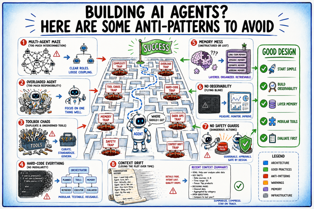
In this article, you will learn the architectural and operational anti-patterns that cause AI agent projects to fail, and how to avoid each one. Topics we will cover include: Why agent failures compound differently than failures in simpler, single-response AI systems. The architectural anti-patterns — from premature multi-agent systems to tool sprawl, hardcoded logic, and missing memory design — that make agents brittle as they scale. The operational anti-patterns — including missing observability, ungoverned write access, context drift, and skipped evaluation — that only surface once an agent reaches production. Introduction AI agents fail in predictable ways. The model is rarely the problem; the architecture, the memory design, the tooling decisions, and the way complexity gets introduced are where things go wrong. Most failed agent projects share a handful of structural mistakes that only become visible later, when they’re expensive to fix. Understanding what breaks AI agents — and why — gives you a better mental model for what working agents actually require. An effective approach is to start simple, build for observability, and add complexity only when you can measure the return. The anti-patterns are what happens when teams do the opposite. This article covers: Why agents fail differently from simpler AI systems The architectural mistakes that compound as your system grows The operational mistakes that only surface in production A summary table mapping every anti-pattern to its fix Start here before you start building. Why Agent Failures Hit Harder A language model answers a question. An agentic system solves a task: assessing what to do, choosing tools, acting on results, adjusting when something goes wrong. The reasoning loop is what makes agents powerful, and it’s also what makes them fail in ways that a prompt-and-response system never would. When a chatbot gives a bad answer, the conversation ends. When an agent goes wrong mid-task, however, it keeps going. It might call tools with bad parameters, produce outputs that downstream steps depend on, or loop indefinitely because it can’t recognize that it’s stuck. The blast radius of a bad decision grows with every step. Autonomous agents also accumulate state across steps, which means errors compound. An incorrect tool call in step two affects the context available in step five. A stale memory entry shapes decisions three steps later. By the time something looks wrong to the user, the agent may have already taken several incorrect actions based on a faulty initial assumption. This is why agent failures are different in kind, not just degree. Reaching for Multi-Agent Architecture Too Soon The most common architectural mistake is treating sophistication as a goal. Teams read about multi-agent systems, hierarchical orchestrators, and peer-to-peer collaboration, and design toward those patterns before they’ve validated whether a single agent can solve the problem. Multi-agent systems introduce coordination overhead that compounds cost and debugging difficulty in ways that are hard to anticipate upfront. A few questions worth asking before you go multi-agent: Can a single agent with well-designed tools already solve the problem? Have you measured where the single-agent approach actually breaks down? Does the business value justify the token cost and added complexity? Usually, for a first deployment, a single agent does the job. Start with the simplest thing that could work, measure it, and add layers only when the data shows you need them. Building One Agent That Does Everything A single agent configured with fifteen tools, sprawling instructions, and responsibility for wildly different task types will underperform across all of them. Optimizing for one kind of input hurts performance on others, which is why routing inputs to specialized agents — rather than one general-purpose one — tends to produce better results. The fix isn’t always to add more agents. Often a well-scoped single agent with specialized skills outperforms a bloated general-purpose one. Narrow the responsibility first. If that still isn’t enough, then you have a real case for splitting. Letting the Tool List Sprawl Every tool added to an agent’s context is a tool the model has to reason about when deciding what to do next. A large tool surface increases the chance of the model choosing poorly, inflates prompt size, and makes debugging harder because there are more possible paths through any given task. Too many tools, or tools with overlapping purposes, actively distract agents from pursuing efficient strategies. Keep the tool set minimal and purpose-specific: Tools should be discrete, reusable modules with clear, non-overlapping responsibilities If tools share similar functions, namespace them explicitly so the model can distinguish them If you’re adding tools to handle edge cases, that’s a signal the task scope needs to shrink — not that the tool list needs to grow AI agent architecture anti-patterns Hardcoding Logic Instead of Building for Change Agent systems change constantly in production. A prompt that works today gets revised next week as tools get refactored and model updates shift what’s possible. When an agent’s logic is hardcoded into a monolithic implementation rather than composed from separable components, every one of those changes risks breaking something else. Modular design means prompts in centralized configuration, tools as discrete units, and agents assembled from only the components they need for a given task. Skipping Dedicated Memory Design Many teams design agents the same way they design chatbots: pass the conversation in, get a response out. An agent working a multi-step task needs to know what it did two steps ago, whether a tool call succeeded, and what intermediate results it’s carrying forward. Without a deliberate memory design, context window overflow becomes a production incident rather than a design consideration. A layered approach handles this cleanly: Short-term session memory for current task state and recent tool outputs Long-term memory (typically a vector store) for cross-session context and learned patterns Structured logs for auditability and debugging Build this in from the start. Retrofitting a memory architecture onto a deployed agent is genuinely painful and usually results in a partial rebuild anyway. Shipping Without Observability AI agents are usually non-deterministic systems with opaque reasoning processes. When
Access Denied
Access Denied You don’t have permission to access “http://zeenews.india.com/technology/whatsapp-tests-age-verification-feature-in-india-ahead-of-dpdp-act-implementation-3065292.html” on this server. Reference #18.c4f43717.1786123042.63c65233 https://errors.edgesuite.net/18.c4f43717.1786123042.63c65233