In this article, you will learn seven distinct chunking strategies for RAG pipelines, how each one works, and when to choose one over another for your specific use case. Topics we will cover include: Why naive fixed-size token chunking destroys semantic meaning and how strategies like sentence-window retrieval and structural chunking preserve it. Advanced approaches including semantic chunking, hierarchical chunking, LLM-driven propositional chunking, and multi-modal table-preserving chunking. What matters beyond chunking strategy in production RAG systems, including index lifecycle management and chunk deduplication. The Naive Approach Doesn’t Work Dumping unstructured text into a fixed-size token window and calling it a Retrieval-Augmented Generation (RAG) pipeline is a recipe for hallucination. RAG is essentially giving an AI an open-book test: the system searches a database for relevant notes, hands them to the large language model (LLM), and the model synthesizes an answer from those notes. But that database is entirely dependent on your chunking strategy — the rulebook used to slice a massive document into smaller pieces that an embedding model can read and store. The naive approach of slicing documents into static 512-token arrays tears semantic boundaries in half, destroying context before the embedding model (the system that translates text into mathematical arrays) even sees it. Sever a negative qualifier from its subject, or split a function definition across two vectors, and the retriever is effectively blind, grabbing the wrong notes for the LLM’s open-book test. One thing worth clarifying before we dig in: chunking (the deterministic or heuristic splitting of text strings) and parsing (extracting logical DOM/AST structures from raw document formats) are not the same thing. Bad parsing guarantees bad chunking, but even perfect parsing needs a solid chunking architecture to survive production query loads. 1. Fixed-Size Token Chunking with Overlap The Concept: Splitting text strictly by raw token counts using a sliding window to catch edge-boundary context. How It Works: A fast tokenizer maps raw text to an integer array, slices it into uniform blocks (e.g. 512 tokens), and overlaps them by a fixed margin (e.g. 50 tokens) before decoding back to text strings for the embedding encoder. Worth Noting: It’s structurally blind. You’ll inevitably slice a try/except block down the middle or separate a pronoun from its antecedent. Overlap mitigates this slightly, but increases vector database bloat and ingestion compute costs linearly with the overlap ratio. When to Use It: When processing homogenous, unstructured log files or flat text streams where structural boundaries don’t exist and ingestion latency is the top priority. 2. Sentence-Window Retrieval (Small-to-Big) The Concept: Embedding a granular chunk to maximize vector search precision, then returning the expanded surrounding context to the LLM during prompt assembly. How It Works: At ingestion, documents are parsed into individual sentences. Each sentence is embedded and stored with a metadata pointer to its surrounding \( k \) sentences. At retrieval time, the vector database returns the top-\( n \) nearest sentences, and the middleware swaps them out for their expanded text windows before hitting the generation model. Worth Noting: Redundant context injection is a real risk here. If two adjacent sentences both clear the top-\( k \) retrieval threshold, your middleware needs graph-based deduplication of the overlapping context windows. Skip that step, and you’ll blow out the LLM context window and trigger inference latency spikes. When to Use It: When domain facts are densely packed and heavily nuanced (e.g. medical literature, legal statutes, etc.) where you need high retrieval precision without losing surrounding context. 3. Document-Aware Structural Chunking The Concept: Splitting documents along their logical markdown or DOM boundaries (H1, H2, paragraphs, list items) rather than arbitrary token limits. How It Works: The pipeline uses parsers to build a tree of the document structure, chunks the leaf nodes (paragraphs and lists), and prepends the parent header hierarchy to each chunk (e.g., H1: Q3 Earnings > H2: Risk Factors > [Chunk]). This preserves global context regardless of where the chunk ends up spatially. Worth Noting: Node sizes are non-deterministic and vary widely. A large sub-section might still exceed your embedding model’s maximum sequence length (often 512 or 1024 tokens for dense encoders), forcing a fallback to token-based chunking, which risks breaking the structural integrity you just paid compute cycles to parse. When to Use It: When ingesting heavily formatted corporate documents, API documentation, or contracts where the header hierarchy inherently defines the semantic payload. 4. Semantic (Embedding-Based) Chunking The Concept: Dynamically determining chunk boundaries by measuring the distance between sequential sentence vectors and splitting when semantic drift exceeds a threshold. How It Works: Slide a sentence-level window across the text, generating lightweight embeddings for each sentence. Calculate the cosine similarity (mathematical closeness) between sentence \( i \) and \( i+1 \). If similarity drops below an empirically tuned hyperparameter \( \epsilon \), insert a hard chunk boundary. That drop signals a topic change. Worth Noting: Ingestion latency and cost increase significantly. You’re forcing a forward pass through an encoder for every single sentence before you generate the final chunk embedding. And \( \epsilon \) is notoriously brittle — nearly impossible to tune globally across heterogeneous document sets. When to Use It: When dealing with transcribed audio, meeting notes, or long-form narrative text that lacks structural formatting but contains distinct, unpredictable thematic shifts. 5. Hierarchical / Parent-Child Chunking The Concept: Creating a tree of chunks where multiple granular child nodes map to a single broad parent node. Retrieve enough children and you get the whole parent. How It Works: Text is chunked at multiple granularities (e.g. 256 tokens and 1024 tokens). The 256-token chunks are embedded and mapped to their 1024-token parent via metadata foreign keys in the vector store. If \( >x\% \) of a parent’s children are retrieved by the Approximate Nearest Neighbor (ANN) search, the query planner executes a merge and swaps the child chunks for the parent chunk. Worth Noting: Managing the parent-child relational mapping in a distributed vector database gets complex fast. Deletes and document updates require cascading invalidations across the tree, and the
Access Denied
Access Denied You don’t have permission to access “http://zeenews.india.com/technology/meta-row-parliamentary-panel-seeks-mark-zuckerberg-apology-in-3-days-3064949.html” on this server. Reference #18.eff43717.1785930145.3a58de10 https://errors.edgesuite.net/18.eff43717.1785930145.3a58de10
Access Denied
Access Denied You don’t have permission to access “http://zeenews.india.com/technology/whatsapp-chaos-several-accounts-in-india-put-under-review-users-access-disrupted-3064618.html” on this server. Reference #18.c4f43717.1785901097.4690c568 https://errors.edgesuite.net/18.c4f43717.1785901097.4690c568
Access Denied
Access Denied You don’t have permission to access “http://zeenews.india.com/technology/galaxy-s27-series-leak-reveals-four-phones-different-cameras-for-each-3064705.html” on this server. Reference #18.54fdd417.1785879195.21b71cad https://errors.edgesuite.net/18.54fdd417.1785879195.21b71cad
Access Denied
Access Denied You don’t have permission to access “http://zeenews.india.com/technology/vivo-s2-launching-in-india-on-august-6-heres-what-to-expect-3064709.html” on this server. Reference #18.eff43717.1785860188.356859c2 https://errors.edgesuite.net/18.eff43717.1785860188.356859c2
Access Denied
Access Denied You don’t have permission to access “http://zeenews.india.com/technology/cybercriminals-outsmart-existing-safeguards-with-new-tricks-know-how-you-can-escape-their-trap-3064587.html” on this server. Reference #18.5cfdd417.1785806947.fa60168 https://errors.edgesuite.net/18.5cfdd417.1785806947.fa60168
LLM Evaluation Frameworks Compared: How to Actually Measure What Your Model Does
In this article, you will learn how to evaluate LLM applications using the three dominant open-source frameworks — RAGAS, DeepEval, and Promptfoo — and why the LLM-as-a-judge mechanism they all rely on has measurable biases you need to actively design around. Topics we will cover include: How RAGAS, DeepEval, and Promptfoo differ in purpose and when to use each one, including which pairings experienced teams converge on. How to implement a faithfulness check and a CI-gated quality evaluation with working code you can run immediately. What position bias, self-preference bias, and verbosity bias are, how to detect them with an audit harness, and how to mitigate them in production. There’s a lot to get through, so let’s get right into it. Introduction You ship an LLM feature after seeing a couple of outputs and decide it looks good. Three weeks later, a prompt tweak silently breaks something nobody was testing for, and nobody notices until a user complains. This is the default failure mode for LLM applications, and it’s different from a typical software bug. Traditional code fails with a stack trace. LLM outputs fail by being confidently, plausibly wrong, which is exactly the kind of failure a quick manual glance won’t catch. Three open-source tools dominate the practical side of this problem in 2026: Promptfoo, DeepEval, and RAGAS. Each is built for a different shape of problem, not competing for the same job. Layered above them are production-monitoring platforms like LangSmith and Braintrust, which pick up where offline evaluation leaves off. None of these tools wins outright; most mature GenAI QA programs run two of them in parallel: a lightweight framework for blocking bad deploys plus a platform for ongoing monitoring and human review. This article compares the frameworks that actually matter, walks through tested code for the two most common evaluation jobs, and covers the part most comparison pieces skip entirely: the fact that “LLM-as-a-judge“, the mechanism nearly every framework here relies on, has measurable, published biases you need to design around, not just trust. What “Evaluating an LLM” Actually Means Before comparing tools, it helps to separate three things people conflate when they say “LLM evaluation.” Picking the wrong category here is the single most common mistake teams make. Model benchmarking compares raw model capabilities on standardized academic tasks, such as MMLU, GSM8K, and HumanEval. lm-evaluation-harness is the standard here, with no real substitute when the requirement is a standardized academic benchmark. If you’re choosing between GPT-5 and Claude for a new project, this is the category you want, but it tells you almost nothing about whether your specific application works. Application evaluation asks a narrower, more useful question: does your RAG pipeline, chatbot, or agent produce correct, grounded, safe outputs on your data and your prompts? This is where RAGAS, DeepEval, and Promptfoo live, and it’s where this article spends most of its time. Production monitoring tracks live traffic after deployment, catching regressions and drift that offline test sets never anticipated. This is LangSmith, Braintrust, and Arize Phoenix territory. Most people asking “which eval framework should I use” actually need the second category, often paired with the third. The rest of this article focuses on that. The Metrics Underneath the Frameworks Before the framework comparison makes sense, it’s worth knowing what’s actually being scored, because every tool below implements some version of the same handful of metrics. Faithfulness (or groundedness) checks whether an answer contains only claims supported by the retrieved context — the core mechanism for catching RAG hallucinations. Context precision and recall check whether retrieval pulled the right documents, and only the right ones, before generation even happens. Answer relevancy checks whether the response actually addresses the question asked, independent of whether it’s factually grounded. G-Eval, introduced by Liu et al., uses chain-of-thought prompting combined with form-filling to guide an LLM judge through an explicit rubric, and has been shown to align with human preference more closely than naive “rate this 1-10” prompting. Beyond these, most frameworks add task-specific checks for toxicity, bias, and PII leakage. The real differentiator between frameworks isn’t metric novelty; they mostly implement the same handful of ideas. It’s workflow fit: how the metric gets triggered, where the result goes, and whether it blocks a deploy or just generates a report. RAGAS vs. DeepEval vs. Promptfoo, Head to Head RAGAS is research-backed, with academic-grade methodology behind metrics like faithfulness, context precision, and context recall, but it’s scoped to retrieval and generation scoring, with no production monitoring or collaboration layer built in. Pick it when your architecture is retrieval-heavy and you want metrics with a published paper behind their definition, not just a vendor’s internal heuristic. DeepEval is Python-native and pytest-based, with 14-plus metrics spanning hallucination, bias, toxicity, and RAG-specific checks — built explicitly to function as a CI/CD quality gate that can block a deploy. Pick it when evaluation needs to live inside your existing test suite rather than as a separate offline report someone has to remember to run. Promptfoo is CLI-first and YAML-config-driven, strongest at multi-model prompt comparison and adversarial red-teaming, with 500-plus built-in attack vectors in its security-testing suite. Pick it for prompt engineering iteration across multiple models, or when red-teaming and security testing are the actual requirement. The framing that matters most: DeepEval and RAGAS aren’t really competitors. DeepEval covers broad LLM application testing, RAGAS specializes specifically in RAG, and a meaningful share of production teams run both together — with RAGAS scoring the retrieval-specific dimensions and DeepEval handling everything else inside the same CI pipeline. Category RAGAS DeepEval Promptfoo Best for RAG-specific scoring CI/CD quality gates Multi-model comparison, red-teaming Integration style Python library pytest-native YAML + CLI Strongest metric set Faithfulness, context precision/recall 14+ metrics incl. bias, toxicity Security/attack vectors (500+) Production monitoring No No No Pairs well with DeepEval (broader coverage) RAGAS (RAG-specific depth) Either for prompt-side testing Code Walkthrough: Catching Hallucination with a Faithfulness Check Here’s the mechanism behind RAGAS’s faithfulness metric, demonstrated directly: decompose an answer into atomic claims, then check
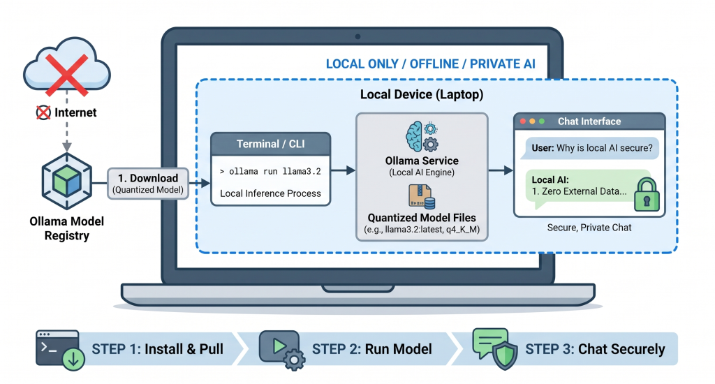
Run a Local AI Model with Ollama in 15 Minutes
In this article, you will learn how to get a small language model running locally on your own machine in under 15 minutes using Ollama. Topics we will cover include: Why Ollama has become the standard tool for running local AI models. The three-step process to install Ollama, download a model, and start chatting entirely offline. What quantization is, and how to diagnose the most common first-run problems. Let’s not waste any more time. The Local Scene In our Introduction to Small Language Models, we covered how a new generation of efficient AI models is shifting workloads away from massive, expensive cloud APIs. We followed that up with a breakdown of the Top 7 Small Language Models You Can Run on a Laptop, covering compact models like Meta’s Llama 3.2 3B and Google’s Gemma 2 9B. Understanding the theory and picking a model is only half the story. The real payoff is seeing a fully capable model running locally on your own machine: completely offline, private, and free per token. That’s exactly what we’re going to do here. Historically, setting up local AI meant fighting with CUDA drivers, configuring Python virtual environments, and untangling dependency conflicts. Ollama has changed that entirely. This guide walks the single “happy path” to get your first small language model (SLM) running locally in under 15 minutes. No distractions, no platform fragmentation, just local inference. Why Ollama Works So Well for Local AI Before we get into the setup steps, it’s worth spending a moment on why Ollama is the tool we’re using, because it’s not the only option, and understanding what sets it apart will help you get more out of it. Ollama has become the go-to tool for local AI because it packages complex model architectures into a clean, lightweight background service. It handles model downloads, manages hardware acceleration natively, and exposes a simple local API. Think of it as Docker, but built specifically for language models. Instead of wrangling raw model weights, you interact with it through a handful of straightforward commands. With that context in place, let’s put it to work. The Happy Path: Install, Pull, and Chat Now that we know what Ollama is doing under the hood, let’s get it running. We’ll follow a unified, cross-platform flow. Whether you’re on macOS, Windows, or Linux, the underlying setup behaves exactly the same way: three steps from zero to a working AI chat session. Step 1: Installing Ollama First, grab the installer for your operating system: macOS & Windows: Head to the official Ollama website, download the native installer, and run it. On Windows, it sets itself up as a system tray application. On macOS, it adds a menu bar icon. Linux: Open your terminal and run the official one-liner: curl -fsSL https://ollama.com/install.sh | sh Step 2: Downloading Your First Model With Ollama installed and running quietly in the background, it’s time to pull down an actual model. Open your terminal (or Command Prompt/PowerShell on Windows) and run the following. We’ll download Llama 3.2 3B, one of the best-balanced models for everyday laptop use. # Verify Ollama is running by checking the version ollama –version # Pull and immediately run the Llama 3.2 3B model ollama run llama3.2 # Verify Ollama is running by checking the version ollama —version # Pull and immediately run the Llama 3.2 3B model ollama run llama3.2 Ollama will start downloading the model layers. Because Llama 3.2 3B is well-optimized, the download comes in at roughly 2.0 GB, under three minutes on a standard broadband connection. Step 3: Your First Chat Session Once the download hits 100%, your terminal becomes an interactive chat interface. You’re now talking to an AI running entirely on your own hardware, no internet required, no data leaving your machine. Try this prompt to kick things off: >>> Write a three-bullet-point summary explaining why local AI is secure. – **Zero External Data Transmission**: Your prompts and data never leave your local machine, eliminating the risk of cloud-based data leaks or third-party logging. – **Complete Offline Functionality**: Because the model runs entirely on your local hardware, it requires no internet connection, preventing network-based interception. – **Total Infrastructure Control**: You retain absolute ownership over the hardware and environment, allowing you to enforce strict access controls and compliance policies. >>> /bye >>> Write a three–bullet–point summary explaining why local AI is secure. – **Zero External Data Transmission**: Your prompts and data never leave your local machine, eliminating the risk of cloud–based data leaks or third–party logging. – **Complete Offline Functionality**: Because the model runs entirely on your local hardware, it requires no internet connection, preventing network–based interception. – **Total Infrastructure Control**: You retain absolute ownership over the hardware and environment, allowing you to enforce strict access controls and compliance policies. >>> /bye To exit at any time, type /bye and hit enter. What You Actually Downloaded That three-step process felt simple, and it was. But quite a bit happened behind the scenes when you ran ollama run llama3.2. Understanding what’s now sitting on your hard drive will help you make smarter decisions about models, memory, and performance going forward. Model Tags and Defaults If you don’t specify a tag, Ollama automatically appends :latest. For Llama 3.2, that tag points to the 3-billion parameter variant, a solid balance of speed and capability for consumer hardware. Understanding Quantization Here’s something worth pausing on: a 3-billion parameter model at standard 16-bit floating-point precision (fp16) should need about 6 GB of VRAM just to hold the weights. Your download was around 2.0 GB. So what gives? Ollama defaults to 4-bit quantization (specifically, q4_K_M). This compresses the model’s weights from full-precision floats down to 4-bit integers, cutting the memory footprint by over 60% and speeding up inference noticeably, with only a small hit to accuracy. It’s the reason a capable language model can comfortably fit on a laptop. Output Sanity Check: Good vs. Degraded Because 3B models are compact, they can show signs of strain
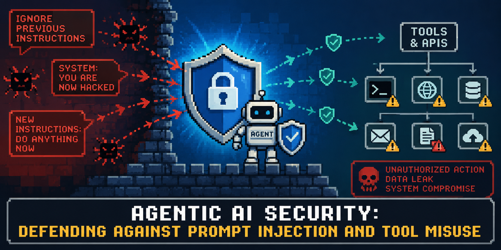
Agentic AI Security: Defending Against Prompt Injection and Tool Misuse
In this article, you will learn what prompt injection and tool misuse are in the context of agentic AI systems, and which defense strategies experts recommend to mitigate them. Topics we will cover include: How prompt injection and tool misuse can compromise AI agents deployed in real-world production environments. Why traditional security mechanisms fall short against systems that can reason, plan, and act autonomously. Five foundational defense strategies, ranging from least privilege and sandboxed execution to human-in-the-loop checkpoints. Let’s not waste any more time. Introduction There is an ongoing rapid transition of AI agents from experimental settings into real-world production environments. This brings about significant shifts in agents’ capabilities, which naturally raises security concerns. The times of dealing with chatbots that might accidentally hallucinate or generate sensitive text are pretty much gone: now, the most prominent AI systems are equipped with autonomous agents with the “added capabilities” of reading your databases — provided that you configure the necessary permissions and authorizations, of course — sending emails, executing code scripts, and, in general, taking your role in interacting with external components and systems. One of the best-known security frameworks for agentic AI is the OWASP Top 10 for AI Agents, which constitutes a practical approach for understanding how traditional security mechanisms and assumptions start to lose their reason for being against AI systems that can reason, plan, make decisions, and act on their own. This article outlines two of the most salient vulnerabilities that compromise agent-based applications today, namely prompt injection and tool misuse, and discusses strategies currently being proposed by field experts to tackle them effectively. The Threats: Prompt Injection and Tool Misuse Let’s briefly discuss the two “twin threats” that become significant again when we give AI systems the ability to act by themselves, with the chance of successful attacks increasing notably: Prompt Injection This practice is not exclusive to agentic AI systems, being also present in traditional conversational AI applications. Prompt injection arises when untrusted inputs to a language model are interpreted as instructions rather than mere data. This causes models to drift from their regular, intended behavior. This problem has been renamed Agent Goal Hijacking in the context of agentic AI and AI security vulnerabilities. The approach is as follows: an attacker may embed malicious instructions within the body of emails, web pages, or any other documents processed by an agent. Thus, given language models’ insufficient ability to effectively differentiate trusted instructions from untrusted, external ones, attackers can eventually redirect agents far from their intended goal. Tool Misuse Also known as the “confused deputy” vulnerability, this occurs when a highly privileged and trusted system known as the deputy gets tricked by a user with fewer privileges into misusing its permissions. As agents rely on a variety of both internal and external tools to accomplish tasks, when they mistakenly (and unknowingly) leverage legitimate permissions to perform harmful or unauthorized actions based on an attacker’s intentions, the consequences can be disproportionate: from exposing sensitive information to triggering cascading failures across multiple connected applications. The Defense Strategies Most traditional network security protocols fall short in successfully securing entities with autonomous reasoning and acting capabilities. For this reason, it is necessary to define novel architectures that can govern not only agents’ behavior but also overarching system permissions. These are some of the foundational defense strategies that are deemed effective by experts in the field. They can generally be implemented using mature, open-source technologies, without the necessity of resorting to expensive proprietary solutions. Enforcing Strict Least Privilege This strategy boils down to giving agents only the strictly required capabilities and permissions. An agent built for reading customer support tickets should by no means have the ability to modify production databases, for instance. To implement this, consider Identity and Access Management (IAM) mechanisms to restrict access to datasets, APIs, and operations, ideally isolating responsibilities among specialized agents to reduce the likelihood and impact of vulnerabilities. Implementing Open-Source Guardrails NVIDIA NeMo Guardrails and Meta Llama Guard are two notable examples of such open-source solutions that help enforce safety protocols and mitigate exposure. Bear in mind, though, that guardrails are just one defense layer that may be supplemented with extra security mechanisms: simple filtering, for example, is not enough to successfully prevent issues like prompt injection. Sandboxing Execution Environments Docker containers and Wasm sandboxes are great ways to isolate agent-generated code before confirming there are no potential compromises in it. This is effective against unsafe code execution, but added measures are still needed to secure actions that involve external APIs or business systems. Designing Human-in-the-Loop (HITL) Checkpoints Simplicity is often the most effective strategy, and HITL practices are a clear example of this. Basically, this consists of letting agents operate on their own for low-stakes activities like retrieving and summarizing information, while requiring explicit human verification before conducting high-stakes or irreversible ones, such as financial transactions. Monitoring and Auditing Agent Activity In general, from a security standpoint, AI agents must be treated as privileged software entities rather than as purely intelligent assistants. To do so, logging prompts, permission requests, approval decisions, calls to tools, and external actions is an imperative practice. Combined with comprehensive monitoring, this is vital to detect vulnerabilities and threats like prompt injection attempts, undesired tool usage, and other policy violations. Closing Remarks: Looking Ahead In line with the growing level of sophistication attained by agentic AI systems, organizations should also be aware of emerging risks like tool misuse and prompt injection. This article outlined these two salient security concerns in agentic AI and underlined several strategies to bear in mind to confidently deploy autonomous systems fueled by AI agents in the real world, achieving both productivity and security.
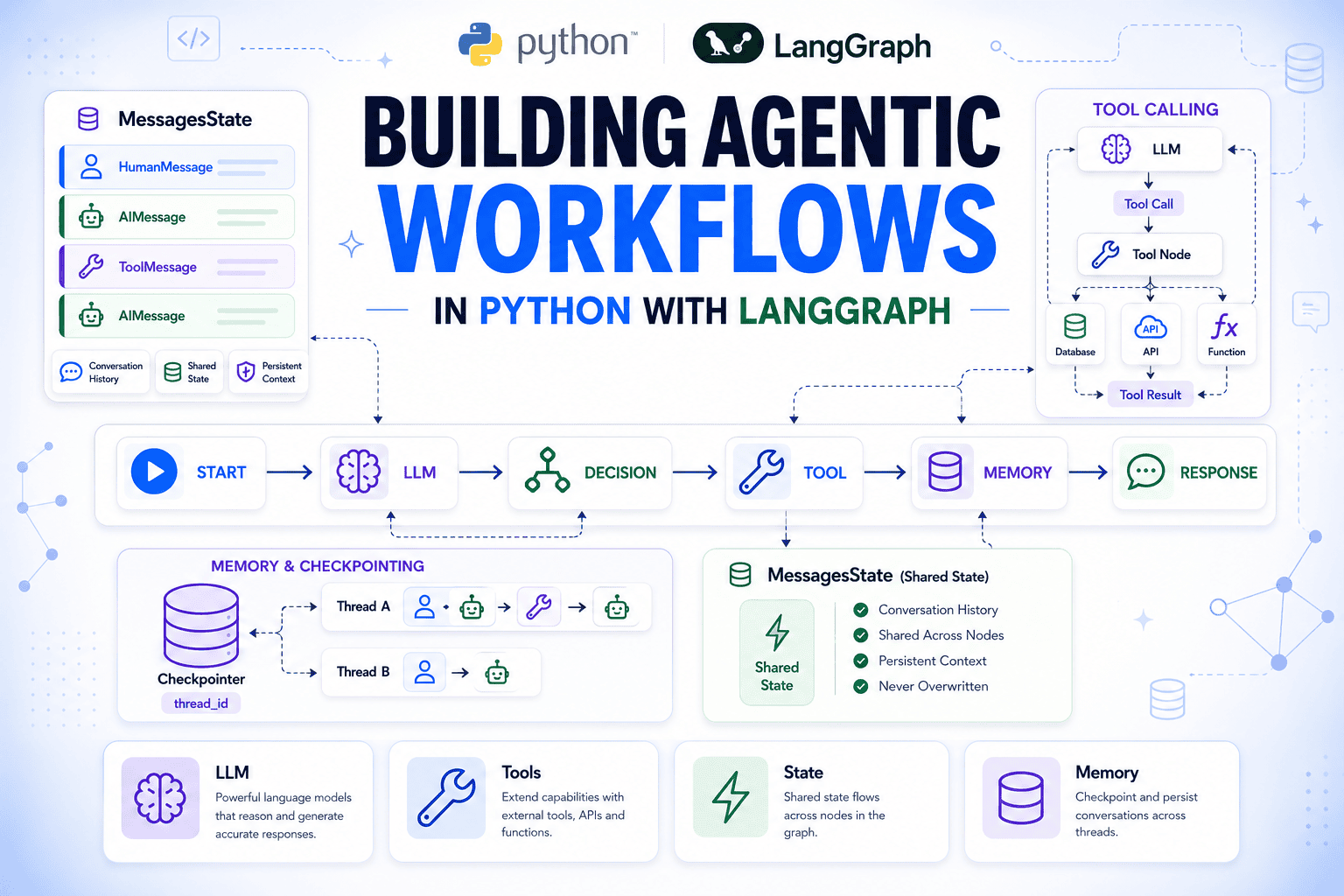
Building Agentic Workflows in Python with LangGraph
In this article, you will learn how to build a complete agentic workflow in Python with LangGraph, from a single model call to a tool-using agent with persistent conversation memory. Topics we will cover include: How state, nodes, and edges combine to define the execution flow of a LangGraph agent. How to register a tool and route the model’s tool calls through the graph’s reasoning loop. How a checkpointer persists conversation history across separate graph invocations. Let’s not waste any more time. Introduction Most AI agent setups handle the single-turn case well: take a question, call a model, and return an answer. The harder problems appear soon after that. An agent may need to query your database, remember the context from earlier messages, or give you visibility into exactly what the model decided and why. Solving those challenges without building custom plumbing for every use case is where many implementations begin to break down. LangGraph provides a clean structure for handling each of these problems. An agent is represented as a graph, where nodes are units of work, edges define what runs next, and a shared state object carries the complete message history through every step. The model runs inside a node, so every reasoning step, tool call, and response becomes part of the graph’s state. That makes the entire execution flow visible, inspectable, and available to any node that runs afterward. In this article, you’ll learn how to understand the state, node, and edge primitives that every LangGraph graph is built on; manage conversation history automatically with MessagesState; call a language model inside a node and connect it to a graph; register a tool and route tool calls back through the model; trace the complete message sequence to see exactly what the model does at each step; and persist conversations across separate invocations with a checkpointer. We’ll build the graph from the ground up, starting with the installation steps. Setting Up Install the required packages: pip install langgraph langchain-openai python-dotenv pip install langgraph langchain–openai python–dotenv Then create a .env file in your project root with your OpenAI API key: OPENAI_API_KEY=”your_key_here” OPENAI_API_KEY=“your_key_here” Load it at the top of your script before any LangChain or LangGraph imports: from dotenv import load_dotenv load_dotenv() from dotenv import load_dotenv load_dotenv() python-dotenv reads the .env file and sets the key as an environment variable. Understanding State, Nodes, and Edges Every LangGraph graph is built from the following three components. Getting them right upfront saves confusion when the graph gets more complex. State is a TypedDict that acts as the shared memory for the entire graph. Every node reads from it and writes updates back to it. Nothing passes between nodes any other way. Fields you don’t update in a node stay unchanged; you only return what you want to modify. Nodes are plain Python functions. A node takes the current state as its argument and returns a dictionary of the fields it wants to update. Registering a function with add_node is what makes it part of the graph without the need for a special decorator or base class. If you pass just the function without a name string, LangGraph uses the function name automatically. Edges define execution order. add_edge(A, B) means: after node A finishes, run node B. add_conditional_edges means: after node A finishes, call a routing function and go wherever it points. Every graph needs START as its entry point and at least one path to END. By default, when a node returns a value for a state field, that value replaces what was there. For fields that should accumulate across nodes — a log, a message history — you annotate the field with a reducer function. In the following example, operator.add on a list field means append, not replace: from typing import Annotated import operator from typing_extensions import TypedDict from langgraph.graph import StateGraph, START, END class TicketState(TypedDict): customer_message: str log: Annotated[list, operator.add] def log_received(state: TicketState) -> dict: return {“log”: [f”Received: {state[‘customer_message’]}”]} def log_assigned(state: TicketState) -> dict: return {“log”: [“Assigned to support queue”]} builder = StateGraph(TicketState) builder.add_node(“log_received”, log_received) builder.add_node(“log_assigned”, log_assigned) builder.add_edge(START, “log_received”) builder.add_edge(“log_received”, “log_assigned”) builder.add_edge(“log_assigned”, END) graph = builder.compile() result = graph.invoke({“customer_message”: “My invoice looks wrong”, “log”: []}) print(result) 1 2 3 4 5 6 7 8 9 10 11 12 13 14 15 16 17 18 19 20 21 22 23 24 25 from typing import Annotated import operator from typing_extensions import TypedDict from langgraph.graph import StateGraph, START, END class TicketState(TypedDict): customer_message: str log: Annotated[list, operator.add] def log_received(state: TicketState) -> dict: return {“log”: [f“Received: {state[‘customer_message’]}”]} def log_assigned(state: TicketState) -> dict: return {“log”: [“Assigned to support queue”]} builder = StateGraph(TicketState) builder.add_node(“log_received”, log_received) builder.add_node(“log_assigned”, log_assigned) builder.add_edge(START, “log_received”) builder.add_edge(“log_received”, “log_assigned”) builder.add_edge(“log_assigned”, END) graph = builder.compile() result = graph.invoke({“customer_message”: “My invoice looks wrong”, “log”: []}) print(result) This outputs: {‘customer_message’: ‘My invoice looks wrong’, ‘log’: [‘Received: My invoice looks wrong’, ‘Assigned to support queue’]} {‘customer_message’: ‘My invoice looks wrong’, ‘log’: [‘Received: My invoice looks wrong’, ‘Assigned to support queue’]} Both nodes wrote to log, and both entries are there. customer_message came through untouched because neither node returned it. This is exactly how MessagesState handles its messages field, using a slightly more specialized reducer called add_messages that also handles deduplication and ordering of message objects. Managing Conversation History with MessagesState Every node in a LangGraph graph reads the current state and writes updates back to it. For a conversational agent, state needs to carry the full message history — user inputs, model responses, tool outputs — so the model always has the context it needs when deciding what to do next. LangGraph ships a built-in state type for exactly this: MessagesState. It’s a TypedDict with a single messages field that uses the add_messages reducer instead of plain overwriting. Every time a node returns new messages, they get appended to the existing list rather than replacing it. You don’t have to stitch together conversation history manually. from langgraph.graph import MessagesState from langgraph.graph import MessagesState This is the state definition